
7. Banking Crises and Financial Instability
A banking crisis is more than a fall in bank share prices or the failure of a badly managed institution. It becomes systemic when distress threatens a substantial part of the financial system and disrupts its ability to provide payments, liquidity and credit. The same transformations that make banking useful create vulnerabilities: long-lived, risky and illiquid assets are financed with claims that customers expect to redeem promptly and at a predictable value. History therefore connects the organisation of banks with macroeconomic outcomes. The task is to identify the original shock, the mechanisms that amplify it and the policies that can restore intermediation without preserving unsustainable business models.
Five episodes illustrate different combinations of these mechanisms: the American savings-and-loan crisis; the Nordic crises; Japan's post-bubble banking problems; the global financial crisis of 2007–2009; and the interest-rate and property-market stress associated with the inflation and monetary-tightening cycle of 2022–2023. Their differences matter as much as their similarities. A duration loss, an insolvent borrower and a wholesale-funding run require different immediate responses, even though they can ultimately produce the same contraction in credit.
Identifying a systemic banking crisis
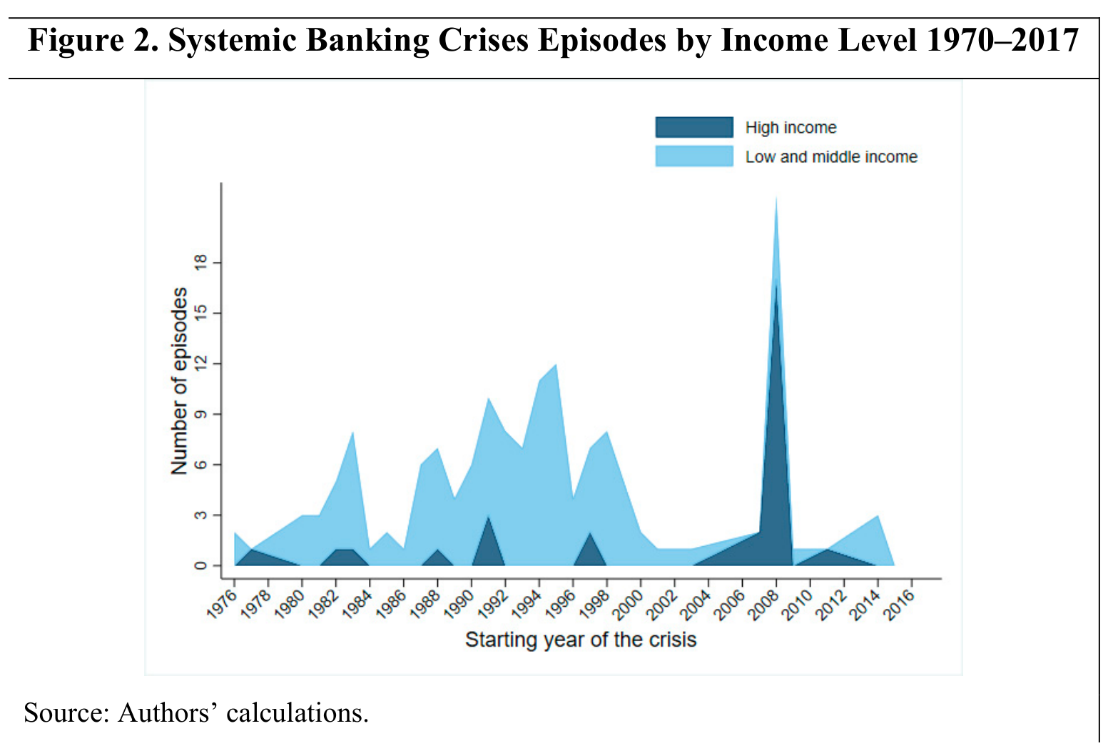
Laeven and Valencia's historical database identifies 151 systemic banking-crisis episodes worldwide during 1970–2017, including borderline cases. This is a count of country episodes, not a count of failed banks or independent global shocks. Several countries can enter crisis in the same international wave. Income classifications refer to countries' income at the start of each episode, using the World Bank's historical thresholds; classifying every observation by its present income would change the comparison.
The normal identification rule combines two conditions: substantial financial distress, evidenced by bank runs, banking losses or liquidations, and substantial policy intervention responding to that distress. The crisis starts in the first year when both conditions are met. There is an important severe-loss exception: very large observed losses or liquidations are sufficient even without three intervention measures. Specifically, the authors use non-performing loans above 20% of total loans, closures covering at least 20% of banking assets, or bank-restructuring fiscal costs exceeding 5% of GDP as indicators of sufficiently severe distress. These are research classification thresholds, not legal triggers for closing a bank.
| Intervention | Operational meaning in the historical database | Economic purpose and limitation |
|---|---|---|
| Deposit freeze or bank holiday | Restrictions on withdrawals, or temporary closure of banks | Interrupts a run, but also disrupts payments and access to savings |
| Significant nationalisation | Government takeover of a systemically important institution, including a majority equity stake | Permits restructuring and control; transfers governance responsibilities to the state |
| Bank restructuring expenditure | Gross fiscal restructuring costs of at least 3% of GDP | Restores loss-absorbing resources; gross expenditure differs from eventual net cost |
| Extensive liquidity support | Support exceeds 5% of deposits and liabilities to non-residents and more than doubles relative to its pre-crisis level | Relieves immediate refinancing pressure; cannot by itself repair negative economic equity |
| Significant guarantees | Broad government protection of liabilities, including protection extended to non-deposit bank liabilities | Restores confidence while creating contingent public exposure; a simple increase in deposit-insurance coverage does not qualify by itself |
| Significant asset purchases | Purchases by public authorities or their agencies exceeding 5% of GDP | Removes or funds troubled assets; the purchase price determines how losses are shared |
Normally, at least three of these six measures establish the intervention condition. The thresholds deliberately exclude minor failures and precautionary interventions that do not accompany systemic distress. However, the approach is not free from measurement difficulties: loss recognition can be delayed, non-performing-loan definitions differ, and a strong early response can reduce observed losses. Alternative databases use historical narratives, bank-equity price declines or credit and output contractions. A result about crisis frequency must therefore state which definition and observation period it uses.
Historical definitions, figures and comparisons in this section are from Laeven and Valencia, Systemic Banking Crises Revisited, IMF Working Paper 18/206 (2018). They describe 1970–2017 and do not constitute an inventory of subsequent banking events.
Crisis waves, currency pressure and sovereign debt
Banking crises occur in clusters rather than at a constant annual rate. The Latin American debt problems of the early 1980s, the transition from centrally planned economies, the Mexican crisis, the Asian crisis and the global financial crisis generated visible international waves. High-income economies were affected by the American savings-and-loan crisis, Nordic failures and Japan's crisis before 2007, but the global financial crisis greatly increased their representation in the dataset. The apparent calm of the mid-2000s was therefore poor evidence that severe banking instability had disappeared.
A currency crisis in this database requires a year-on-year depreciation against the US dollar of at least 30%, with the depreciation rate at least 10 percentage points higher than in the previous year. For repeated qualifying depreciations, the authors use the first year within a five-year window; early transition episodes are excluded. Sovereign-debt crises are dated using defaults to private creditors and/or restructurings. A twin crisis combines banking distress in year with a currency or sovereign crisis in ; a triple crisis includes both. These conventions prevent every exchange-rate movement or public-debt increase from being called a separate crisis.
| Banking-crisis category | Episodes | Share of banking episodes |
|---|---|---|
| Banking crisis without a currency or sovereign crisis in the overlap window | 107 | 70.9% |
| Banking and currency crisis, without sovereign crisis | 31 | 20.5% |
| Banking and sovereign crisis, without currency crisis | 2 | 1.3% |
| Banking, currency and sovereign crisis | 11 | 7.3% |
| All banking episodes | 151 | 100.0% |
The counts imply 107 standalone banking episodes and 44 overlapping episodes, so the overlapping share is . A country can experience banking distress without either of the other two crisis types. Nevertheless, the connections are powerful. A currency depreciation increases the domestic-currency burden of foreign-currency debt; bank rescues can weaken sovereign finances; and losses on sovereign bonds can impair banks that hold them. Depositors fleeing domestic banks may also move into foreign assets, adding exchange-rate pressure. In the historical sample, currency and debt crises tend to coincide with or follow banking crises, with currency episodes most frequent one year after banking distress begins. Temporal ordering alone does not prove that banking distress caused every subsequent event.
Containment, restructuring and the limits of liquidity support
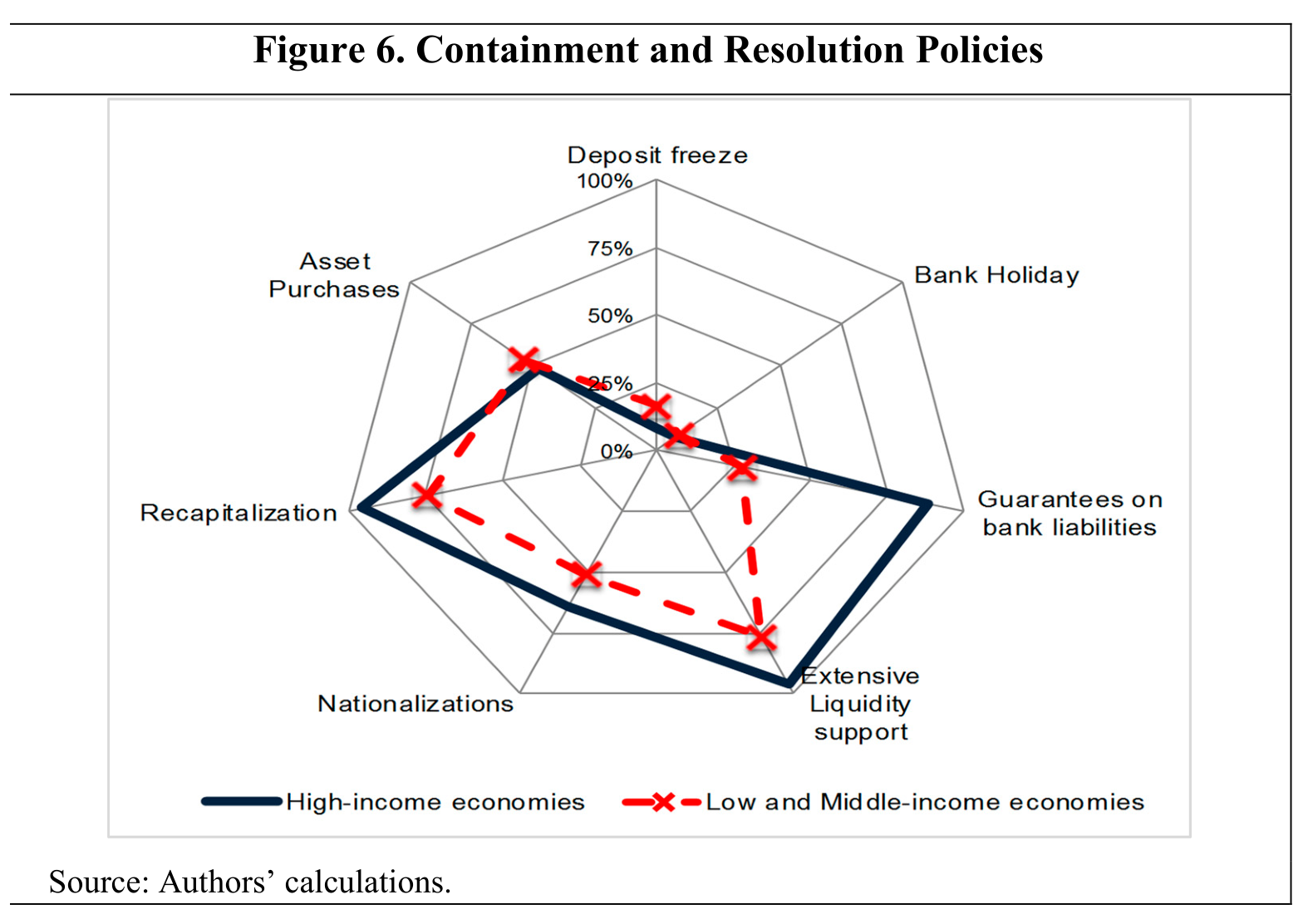
Crisis containment tries to prevent a destructive interruption in payments and funding. Central-bank lending can replace suddenly unavailable private funding, while guarantees can convince creditors to maintain their claims. In the database, peak liquidity support is measured relative to deposits and liabilities to non-residents, rather than relative to GDP. Its median reaches 20.2% across the sample, approximately 12% for high-income economies and 23% for low- and middle-income economies. The increase above the pre-crisis level is a separate measure: its medians are 6.4% and 14.8%, respectively. A large pre-existing reliance on central-bank funds makes the distinction important.
Guarantees were announced in 34 episodes, including 19 in high-income countries. Their credibility depends on the state's fiscal capacity: promising more than the government can plausibly honour may transfer the panic from banks to the sovereign. Guarantees can also remain in force for years after immediate conditions improve. Deposit freezes and bank holidays are more disruptive and were rarer: the study records eight freezes and six bank holidays, with each recorded holiday followed by a freeze. A temporary closure can give authorities time to implement a restructuring, but it is not a way of making underlying losses disappear.
Resolution addresses the allocation of losses and the restoration or orderly withdrawal of banking services. Viable institutions may need new equity, changes in management and business-model repair. Institutions that cannot be made viable need an orderly transfer or wind-down. An asset-management company, often called a bad bank, can separate difficult assets from continuing banking operations and provide specialised recovery expertise. Separation works only if valuations are credible and someone bears the loss: selling a bad loan at an inflated price merely hides a public subsidy. Recapitalisation, asset transfers and nationalisation are distinct instruments, although they can be combined in the same programme.
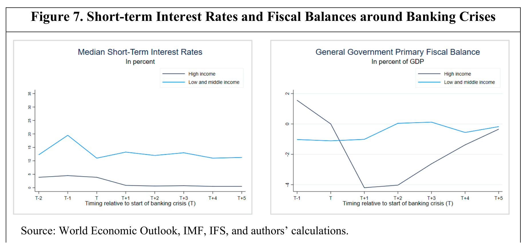
Macroeconomic policy also differs across countries. In high-income episodes, median short-term interest rates fell from around 5% towards zero after the onset of crisis, and primary fiscal balances deteriorated. Lower-income economies were more frequently constrained by currency pressure and access to public borrowing; interest rates could rise and fiscal policy become contractionary. These are historical associations rather than prescriptions. Cutting rates may support domestic demand but aggravate a foreign-currency mismatch if it triggers depreciation. A financial rescue should therefore be evaluated jointly with the monetary, fiscal and exchange-rate constraints under which it operates.
Fiscal expenditure, output loss and the length of recovery
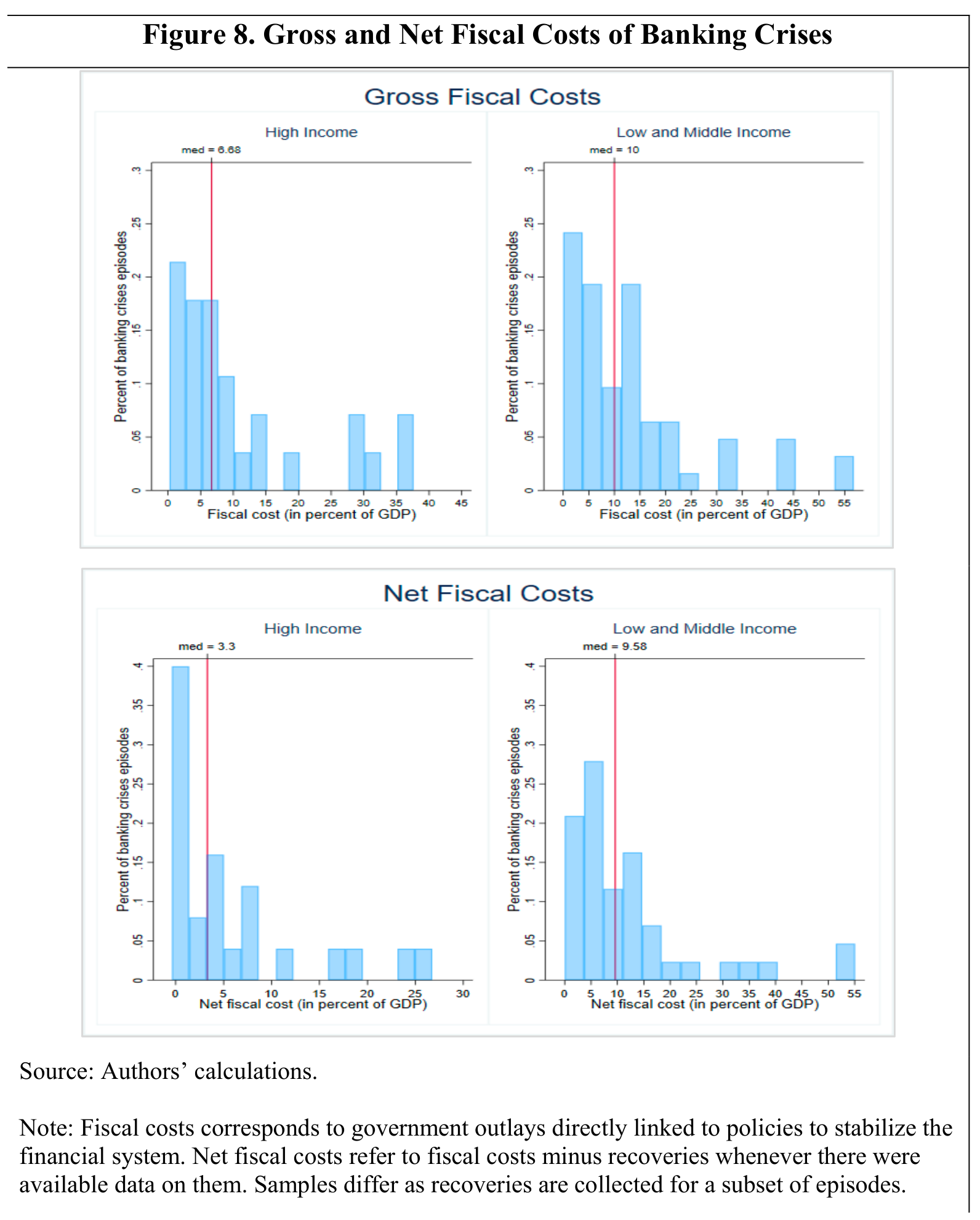
Gross fiscal cost measures public outlays directly associated with financial-sector intervention: capital injections, administrative costs, payments on guarantees that are actually called and other rescue expenditure. An uncalled guarantee is contingent exposure, not an immediate cash expense. Net fiscal cost deducts recoveries such as proceeds from selling acquired assets, dividends, interest and guarantee fees. Unsold assets' unrealised gains are not equivalent to cash recoveries. The historical database divides each year's outlay by that year's nominal GDP and sums those ratios; values expressed relative to financial-system assets use a different denominator and answer a different question.
| Measure | High-income economies | Low- and middle-income economies |
|---|---|---|
| Gross direct fiscal cost, percentage of GDP | 6.7% | 10.0% |
| Net direct fiscal cost, percentage of GDP | 3.3% | 9.6% |
| Increase in public debt, percentage points of GDP | 21.1 | 16.4 |
| Peak non-performing loans, percentage of loans | Slightly above 11% | 30% |
| Duration pattern under the study's convention | More than half last five years or longer | Most last four years or less |
Gross and net medians use different available samples because recoveries are not observed for every episode. Their difference cannot be treated as the median recovery amount. Public-debt increases also include recession-related revenue losses, automatic stabilisers, fiscal stimulus, interest and GDP-denominator effects; they are broader than bank-rescue expenditure. For post-2007 episodes the study compares the change in debt with pre-crisis projections, whereas earlier episodes use the actual change. These distinctions explain why the high-income group can show lower direct rescue costs but a larger rise in public debt.
| Country and crisis start | Gross fiscal cost, % GDP | Net fiscal cost, % GDP | Cumulative output loss, % trend GDP |
|---|---|---|---|
| Finland, 1991 | 12.8 | 11.1 | 69.6 |
| Norway, 1991 | 2.7 | 0.6 | 5.1 |
| Sweden, 1991 | 3.6 | 0.2 | 32.9 |
| Japan, 1997 | 8.6 | 8.5 | 45.0 |
| United States, 2007 | 4.5 | 0.6 | 30.0 |
| Germany, 2008 | 2.7 | 0.7 | 12.3 |
These figures use the database's 2018 information set and measurement conventions. They show why a regional label such as “Nordic crisis” does not imply identical outcomes and why subsequent asset recoveries can materially reduce fiscal cost. The country-level database also records dates, NPLs and policy instruments; those are research observations rather than additional universal crisis rules.
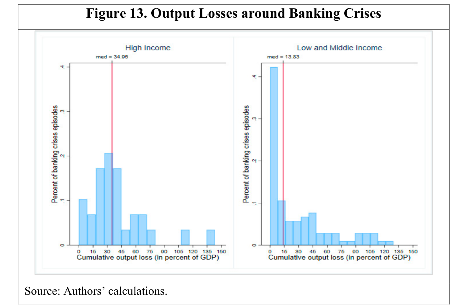
Output loss measures the cumulative shortfall of real GDP from an extrapolated pre-crisis trend during the crisis year and the following three years. The study estimates the trend using a Hodrick–Prescott filter with smoothing parameter 100 on pre-crisis log real GDP, normally using twenty years of history. The four-year cumulative shortfall is expressed relative to a year's trend output. A reported loss around 35% for high-income episodes does not mean that GDP necessarily fell by 35% in a single year: four gaps of roughly 9% would already produce a cumulative figure near that size.
A simple constructed example clarifies the distinction. Suppose the no-crisis path is 100 units of GDP in each of four years and actual output is 94, 90, 91 and 95. The cumulative shortfall is units, or 30% of one year's benchmark output. If government rescue spending is 7 units and subsequent cash recoveries are 4, direct net fiscal cost is 3 units. The economy can therefore suffer a large production loss even when the eventual rescue bill is relatively modest. Neither calculation by itself isolates causation: an energy shock or global trade slump may contribute to the observed output gap.
The historical endpoint of a crisis is the year before real GDP and real credit growth are both positive for at least two consecutive years. When credit data are unavailable, the authors rely on GDP growth. Duration is capped at five years, so a recorded five-year episode means five years or longer, not necessarily full recovery after year five. Credit stocks can remain weak because of loan write-offs even when new lending has resumed. Moreover, positive growth can coexist with output permanently below its earlier path. The paper's output and export profiles show especially persistent shortfalls in high-income economies; many of those observations belong to the global financial crisis, when weak external demand limited recovery through exports.
The savings-and-loan crisis: maturity transformation and delayed recognition
American savings-and-loan associations traditionally financed long-term fixed-rate residential mortgages with shorter-term savings deposits. This business model was vulnerable when inflation and monetary tightening drove market interest rates sharply higher in the late 1970s and early 1980s. New deposit funding became expensive, while old mortgages continued earning low fixed rates. Even before borrowers defaulted, the present value of those mortgages fell. A thrift could consequently have positive historical-cost book capital while the market value of its assets was below its liabilities.
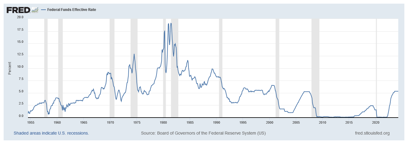
The shock interacted with deposit insurance, regulatory forbearance and deregulation. Allowing a weak institution to continue operating can create an incentive to gamble for recovery: shareholders retain the upside of a successful risky strategy while insured creditors and the public safety net bear much of the downside. Relaxed constraints and weak supervision enabled some institutions to expand into riskier activities instead of repairing their balance sheets. The episode was not simply an unavoidable consequence of high rates; institutional incentives affected the ultimate losses.
The crisis label “1988” in international datasets marks a systemic phase rather than the entire historical sequence. Troubles began earlier, and the Resolution Trust Corporation continued resolving thrifts until 1995. Estimates of outstanding assets, market-value losses and fiscal resolution costs should not be interchanged. The Federal Reserve's historical account reports 747 thrift closures by the RTC, with assets above USD 407 billion, and a taxpayer cost estimated as high as USD 124 billion. A claim that the crisis cost taxpayers USD 600–800 billion would therefore describe a different or inadequately specified quantity.
Two subsequent changes illustrate that risk can move rather than vanish. Adjustable-rate mortgages make the bank's interest income respond to funding rates, reducing some maturity mismatch, but the borrower may then become unable to afford higher payments: interest-rate risk becomes credit risk. Securitisation can transfer mortgages to investors, but weak originator incentives, guarantees and retained exposures may leave risk elsewhere in the banking or shadow-banking system. Risk management must follow the economic exposure through the transaction.
The historical chronology and fiscal-cost distinction are supported by Federal Reserve History, Savings and Loan Crisis, and the FDIC's historical studies of thrift resolution.
The Nordic crises: credit losses and transparent restructuring
Financial liberalisation and rapid lending growth contributed to property and credit booms in Norway, Sweden and Finland during the 1980s. When economic and property-market conditions deteriorated, loans that had appeared safe generated substantial losses. The central vulnerability was aggressive lending and weak asset quality, rather than maturity transformation alone. Loan-loss ratios rose from 0.7% of loans in Norway in 1987 to about 6% in 1991; from 0.3% in Sweden in 1989 to about 7% in 1992; and from 0.5% in Finland in 1989 to about 5% in 1992. These annual loss measures are different from the stock of non-performing loans.
Sweden became an influential example of restructuring because authorities recognised losses, guaranteed relevant bank liabilities, took control of severely distressed institutions and separated troubled assets into asset-management companies. Two large banks, Nordbanken and Gota, became central to the restructuring; their impaired assets were handled through Securum and Retriva. The viable banking operations could continue while specialists worked on asset recovery. Public protection of creditors did not require preserving the value of existing shareholders' investments.
The analytical lesson is the importance of credible recognition and incentives. Independent asset management, transparent valuations and a clear distinction between viable and non-viable institutions reduce pressure to keep bad loans alive. Private owners who can restore viability have an incentive to inject funds before losing control. However, the Nordic countries did not all experience identical policies, costs or recovery speeds. “The Nordic model” describes a family of approaches, and the Swedish institutional details should not be assigned indiscriminately to Norway or Finland.
Country loss ratios and resolution lessons are discussed in Federal Reserve Bank of St. Louis, Resolving a Banking Crisis, the Nordic Way (2009), and the European Commission's study of the Swedish banking-crisis response.
Japan: property collateral, evergreening and a prolonged adjustment
Japan's experience followed a long post-war period without major bank failures. Strong growth, low inflation and financial liberalisation supported optimistic expectations during the 1980s, while lending and collateral valuations became heavily exposed to real estate. The asset-price reversal around 1990 weakened borrowers and banks together. Land pledged as collateral no longer justified earlier loan amounts, and the recognition and disposal of problem loans proceeded slowly. The systemic crisis is dated 1997 in Laeven and Valencia, although important failures, public responses and recapitalisation continued into 1998 and beyond.
Evergreening means extending or renewing funding to a borrower whose underlying repayment capacity is inadequate, often to avoid recognising an existing loss. It differs from a commercially justified restructuring of a temporarily distressed but viable borrower. A bank with little capital may prefer to roll over a bad loan because recognising the loss would reveal that it needs recapitalisation. The strategy can protect reported ratios briefly while tying scarce credit and productive resources to weak firms. Competitors capable of using those resources more efficiently may then receive less finance.
A reported NPL ratio depends on the date, definition and institutions included. A late-1990s figure around 8% and the historical database's 35% peak for the Japanese episode are not reconciled measures with an identical date, definition and institutional perimeter. They should not be spliced into one consistent time series. The mechanism does not depend on choosing whichever statistic looks largest: delayed recognition, weak incentives and unresolved bank capital problems can prolong a credit impairment even when immediate runs are contained. The long period of weak growth often called Japan's lost decade had additional macroeconomic causes; bank distress and capital misallocation were important components rather than a complete explanation.
The global financial crisis: mortgage losses become wholesale runs
Before 2007, rising US house prices supported mortgage borrowing, refinancing and consumption. Prices approximately doubled in some widely used indices between 2000 and 2006, although the exact increase depends on the index and geography. When collateral keeps appreciating, refinancing can conceal weak repayment capacity; lenders and investors may extrapolate unusually favourable default experience. Securitisation broadened the supply of funding but also separated origination from ultimate loss bearing. Fees rewarded transaction volume, complex structures obscured risk, and short-term liabilities financed securities whose liquidity could disappear.
Potential contributing factors include global saving and capital flows, low financing costs, housing-policy incentives, weak underwriting, optimistic ratings, high leverage and the expectation of official support for important institutions. Their relative weight remains debated. It is too strong to explain the entire crisis by one policy or to assume that every mortgage securitisation is inherently defective. The decisive vulnerability was the interaction of common housing exposure with leverage, opacity and runnable finance.
| Period | Selected developments | Mechanism revealed |
|---|---|---|
| First half of 2007 | New Century Financial fails; Freddie Mac tightens its treatment of high-risk mortgages; mortgage and structured-credit losses become visible | Underwriting and valuation assumptions cease to hold |
| Second half of 2007 | IKB requires support involving KfW; asset-backed commercial paper funding contracts; Countrywide and Northern Rock face severe funding pressure | Investors refuse to roll over short-term claims against difficult-to-value assets |
| Early to mid-2008 | JPMorgan acquires Bear Stearns with Federal Reserve assistance; authorities expand liquidity facilities; IndyMac fails in July | Liquidity assistance and assisted transfers attempt to contain contagion |
| September 2008 | Fannie Mae and Freddie Mac enter conservatorship; Lehman Brothers files for bankruptcy; the Reserve Primary Fund breaks the buck; AIG receives emergency support; Washington Mutual fails | Counterparty fears and losses spread across banks, dealers, insurers and money-market funds |
| Late 2008 and thereafter | International interventions expand, including the original USD 700 billion TARP authorisation in the United States | Authorities move from isolated assistance towards system-wide stabilisation and recapitalisation |
Asset-backed commercial paper normally matures quickly. If investors refuse to buy replacement paper, the issuer must obtain alternative liquidity or sell the assets backing it. A run therefore need not involve customers queuing outside a branch. Money-market funds created a related vulnerability: investors expected a stable value and rapid redemption even when underlying securities were risky. After Lehman's failure, losses at the Reserve Primary Fund pushed its net asset value below USD 1 per share, encouraging redemptions and broader pressure on money-market finance. Early redemption can be attractive when later investors bear more of the cost of liquidating remaining assets.
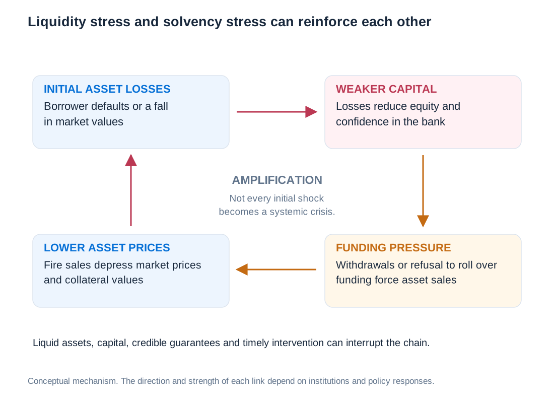
Fire sales connect liquidity and solvency. A sale depresses market prices, reducing collateral values and the measured capital of other holders; lenders demand higher haircuts or more margin; institutions sell further assets. An action that protects one institution can worsen system-wide outcomes. Bank runs are consequently powerful amplifiers, but many historical crises begin with deteriorating assets or unsustainable credit booms. Theoretical self-fulfilling runs remain possible: the historical tendency is not a theorem that panic can never be the initial cause.
The mortgage-credit mechanism and chronology can be compared with Federal Reserve History, Subprime Mortgage Crisis. TARP's original authorisation was a ceiling, not the same quantity as final expenditure or net fiscal loss.
Inflation, monetary tightening and bank fragility in 2022–2023
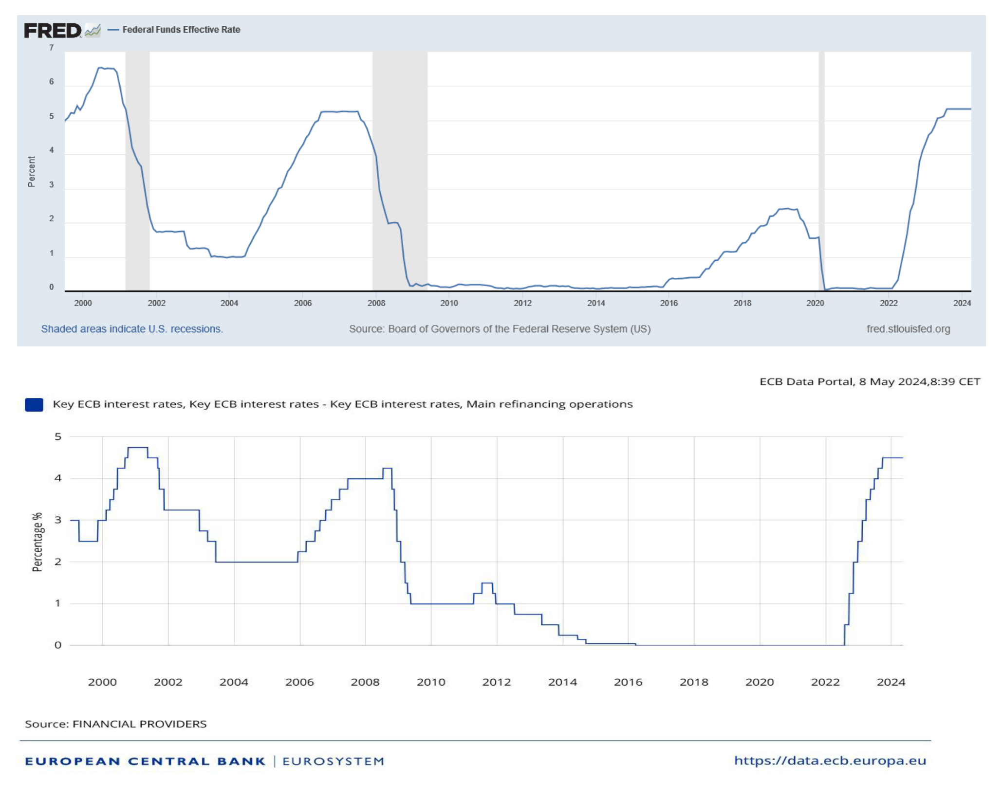
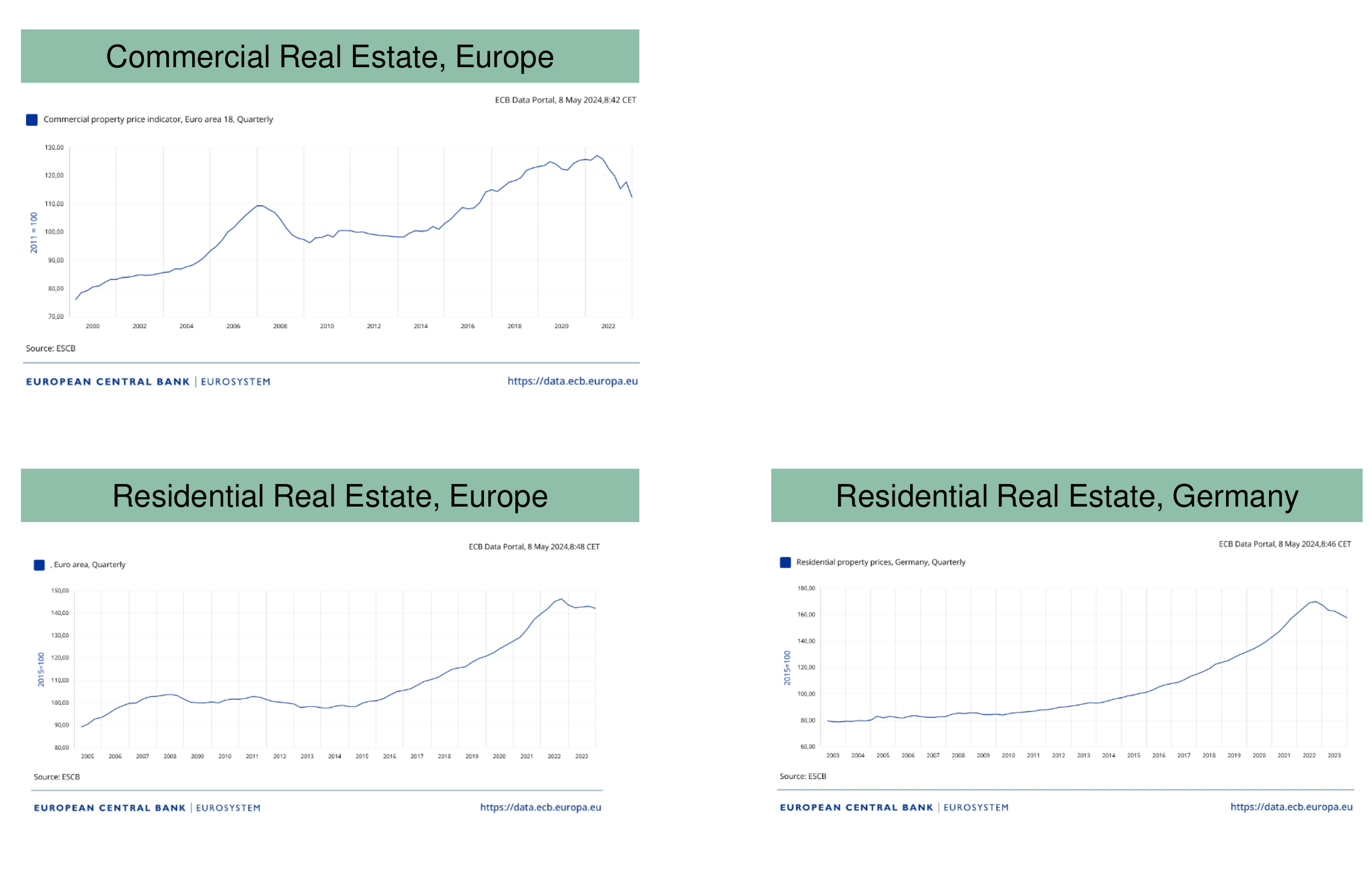
The rise in inflation and subsequent policy tightening exposed a different combination of weaknesses. Long-duration bonds and fixed-rate loans lost market value as discount rates increased. At the same time, real-estate borrowers faced more expensive refinancing and lower collateral valuations. Banks can be exposed through residential mortgages, direct lending to commercial-property companies and property collateral securing loans to other businesses. A government bond with very low default risk can still create substantial interest-rate risk.
For a small parallel yield movement, modified duration provides the approximation
Here is the initial asset value, is modified duration in years, and is the yield change expressed as a decimal. A duration of five years and a two-percentage-point yield increase imply approximately . Convexity, non-parallel yield-curve movements, changing credit spreads and borrower prepayments can materially alter the result. The calculation concerns valuation, not an assumption that 10% of borrowers default.
Funding behaviour determines how that valuation loss affects the bank. Define the deposit beta as the change in the deposit interest rate divided by the change in the relevant market or policy rate. A beta below one means deposit remuneration rises more slowly, supporting the bank's margin and the economic value of its deposit franchise. However, this benefit depends on customers remaining with the bank. Depositors may move to higher-yielding alternatives or withdraw because they doubt the institution's strength. A scenario that marks assets to market and assumes immediate full pass-through to deposit rates is a demanding stress, not a complete going-concern valuation of every bank.
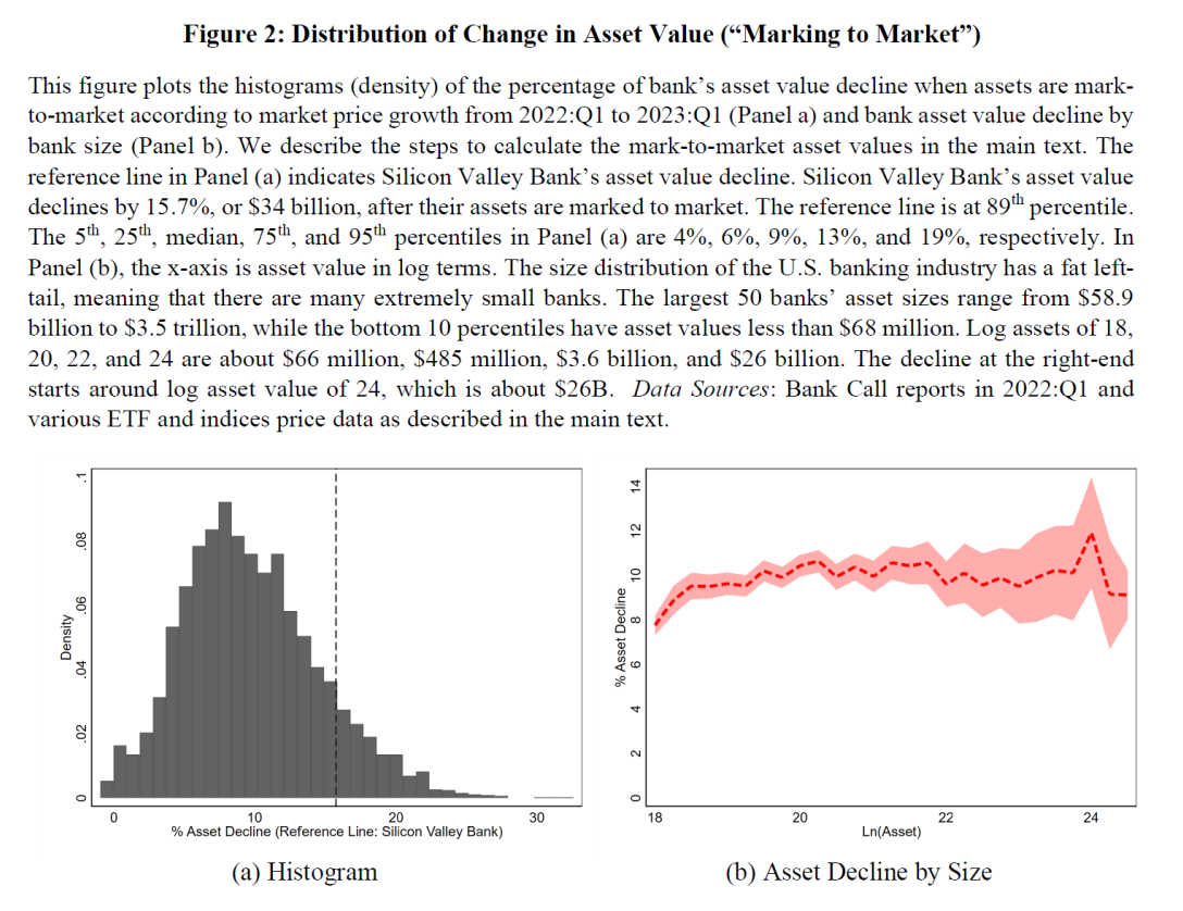
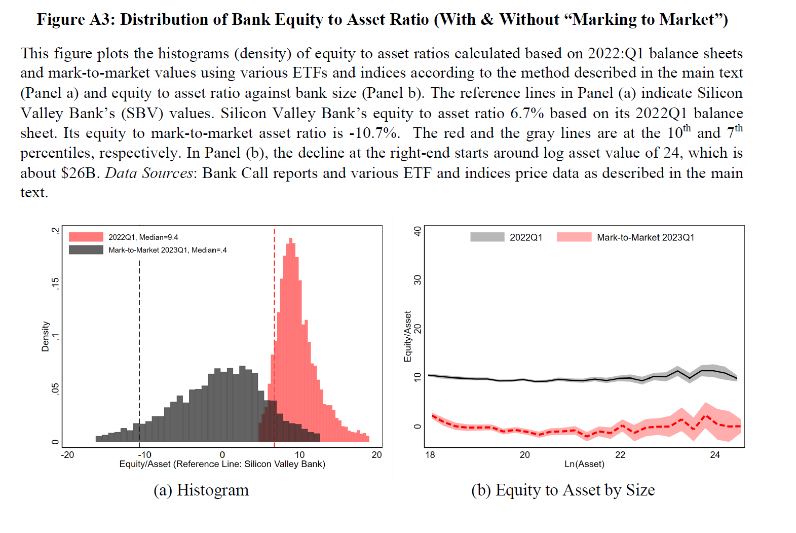
The 2023 analysis by Jiang, Matvos, Piskorski and Seru illustrates the scale of sensitivity when bank assets are revalued after monetary tightening. The distributions and bank-size comparisons identify vulnerability under stated assumptions; they do not mean that every institution with large unrealised losses must fail. Hedging, deposit stability, equity, cash buffers and access to collateralised liquidity matter. Conversely, historical-cost accounting does not guarantee that securities can be held to maturity if withdrawals require an immediate sale.
Silicon Valley Bank's March 2023 failure made this interaction concrete: concentrated uninsured deposits, rapid growth and inadequate management of interest-rate and liquidity risk left the bank exposed to a fast run. The Federal Reserve's April 2023 review also identified supervisory shortcomings. The case supports integrated analysis of assets, funding and governance. It does not establish that all banks with similar accounting losses had the same depositor behaviour or that interest-rate increases alone were sufficient to cause failure.
The bank-valuation figures retain the historical assumptions of Jiang, Matvos, Piskorski and Seru (2023), Monetary Tightening and U.S. Bank Fragility in 2023. The institution-specific account is supported by the Federal Reserve's review of Silicon Valley Bank.
Choosing a response that restores credit allocation
Across these cases, credit booms, collateral optimism and qualitative asset transformation recur. Real estate is especially prominent because exposures are large, assets are long-lived and credit can influence the very prices used to justify additional lending. Deregulation can facilitate valuable competition but also rapid expansion before risk management and supervision adapt. Cross-border funding can support investment and then reverse abruptly. The relevant question is not whether one instrument is always dangerous, but whether the system can bear a common shock without losing its essential functions.
Policy design should begin with credible diagnosis: recognise losses, distinguish viable from non-viable institutions and establish who bears the cost. Prompt recapitalisation and transparent restructuring can allow healthy borrowers to regain access to credit. Indefinite liquidity support for insolvent firms can instead sustain evergreening. Asset-management companies need expertise and independence, and guarantees need an exit strategy. Market-based finance may provide alternative funding when banks retrench, but securities markets themselves can freeze; a diversified system and adequately capitalised banks improve resilience without eliminating every risk.
The three most useful checks are consequently causal. Was the original weakness in duration, underwriting, funding structure or incentives? Which balance-sheet and market mechanisms amplified it? Did the response restore viable intermediation or postpone the recognition of losses? These questions distinguish the Nordic loan-loss episode from the savings-and-loan duration shock, identify wholesale runs during the global financial crisis, and explain why both capital and liquidity regulation are needed.