
4. Loan Pricing, Credit Rationing and Relationship Banking
A bank must earn enough on a loan to compensate for the resources used to originate and service it, the losses expected from default and the funding supplied by depositors and shareholders. However, a higher quoted interest rate is not always a route to a higher expected profit. The rate can change who applies and how a borrower behaves after receiving funds. This chapter connects a transparent pricing calculation to adverse selection, quantity rationing and the value of borrower-specific information.
The economic components of a lending rate
Let be the principal of a simple one-year loan, its operating cost in currency units, its probability of default, the fraction of exposure lost conditional on default, the fraction of funding allocated to equity, the cost of debt funding and the required return on equity. If exposure at default equals principal, a useful additive pricing benchmark is:
All rates and fractions in this equation use the same one-year horizon and are entered as decimals. Multiplication by 100 expresses the resulting rate as a percentage; one basis point is 0.01 percentage point, or 0.0001 in decimal form. The equation treats required annual interest revenue as the sum of operating cost, expected loss and a funding charge. It is a planning decomposition rather than a universal exact cash-flow valuation formula: fees, repayment timing, recoveries, defaulted interest, maturity and the treatment of capital can change the precise contractual rate.
Operating costs include screening the applicant, monitoring performance and collateral, servicing payments and allocated overhead such as systems, premises and management. Some are fixed per account rather than proportional to principal. A EUR 5,000 annual cost is 0.5% of a EUR 1 million loan but 5% of a EUR 100,000 loan. Scale can therefore influence pricing even when borrowers have the same default probability. Allocation also depends on loan type, operational efficiency and which services are shared across the customer relationship.
A break-even estimate answers whether the loan compensates the bank for its costs under stated assumptions. It does not tell the bank what rate it can actually charge. Competition, bargaining, switching costs, differentiated services and information determine the feasible margin. Cross-selling may justify assessing profitability across several services, but an anticipated fee from another product must be a credible economic benefit, not a device for concealing an underpriced loan.
Expected loss, exposure and the meaning of a rating
The basic expected-loss decomposition is:
is an expected monetary loss; is exposure at default; is a default probability for the selected horizon; and is the expected proportion lost after default, including the chosen treatment of recoveries and costs. For revolving commitments, can exceed the current drawn balance if the borrower draws more before failing. For long loans, a one-year PD must not be confused with the probability of ever defaulting over the full maturity. The decomposition also requires consistent assumptions about exposure and severity when these vary with economic conditions.
For euros, and , euros. This is an average over uncertain outcomes, not a prediction that each loan will lose exactly EUR 8,000. Unexpected losses around that average motivate capital and risk limits. An accounting loss allowance and a regulatory capital charge have different objectives and may use different horizons and model constraints, so neither should be equated mechanically with this illustrative one-year calculation.
| Rating family | Illustrative one-year PD range |
|---|---|
| AAA / Aaa | 0.02%–0.03% |
| AA / Aa | 0.03%–0.10% |
| A | 0.10%–0.24% |
| BBB / Baa | 0.24%–0.58% |
| BB / Ba | 0.58%–1.19% |
These ranges are a historical teaching calibration, not a rating agency's permanent promise or a current default forecast. A rating is an ordinal assessment of credit quality. Its empirical default frequency depends on the agency, population, observation period, horizon and definition of default. A better rating does not remove market-price or liquidity risk, and an investment-grade boundary is not a guarantee against loss.
| Ordinal code | Moody’s | S&P | Fitch debt rating | Broad grouping |
|---|---|---|---|---|
| 1 | Aaa | AAA | AAA | Investment grade |
| 2 | Aa1 | AA+ | AA+ | Investment grade |
| 3 | Aa2 | AA | AA | Investment grade |
| 4 | Aa3 | AA− | AA− | Investment grade |
| 5 | A1 | A+ | A+ | Investment grade |
| 6 | A2 | A | A | Investment grade |
| 7 | A3 | A− | A− | Investment grade |
| 8 | Baa1 | BBB+ | BBB+ | Investment grade |
| 9 | Baa2 | BBB | BBB | Investment grade |
| 10 | Baa3 | BBB− | BBB− | Investment grade |
| 11 | Ba1 | BB+ | BB+ | Speculative grade |
| 12 | Ba2 | BB | BB | Speculative grade |
| 13 | Ba3 | BB− | BB− | Speculative grade |
| 14 | B1 | B+ | B+ | Speculative grade |
| 15 | B2 | B | B | Speculative grade |
| 16 | B3 | B− | B− | Speculative grade |
| 17 | Caa1 | CCC+ | CCC+ | Very high credit risk |
| 18 | Caa2 | CCC | CCC | Very high credit risk |
| 19 | Caa3 | CCC− | CCC− | Very high credit risk |
The codes 1–19 merely order the displayed categories. A two-notch change is not twice the default risk of a one-notch change. Nor are the rows exact equivalences between agencies: methodologies and the distinction between issuer and instrument ratings matter. Fitch's debt-rating notches shown here should not be indiscriminately substituted for every issuer or national scale.
| Agency | Label | Interpretation |
|---|---|---|
| Moody’s | Ca | Highly speculative; likely in or close to default, with some recovery prospect |
| Moody’s | C | Lowest category; typically defaulted, with little recovery prospect |
| S&P | CC / C | Extremely weak credit or instrument protection; interpretation depends on the rating type |
| S&P | SD | Selective default at issuer level |
| S&P | D | Default, subject to the relevant issuer or issue definition |
| Fitch | CC / C | Very high default vulnerability / a default-like process beginning |
| Fitch | RD | Restricted default, including specified uncured defaults or distressed exchanges |
| Fitch | D | Default under the relevant rating definition |
An older simplified comparison assigns code 20 to Ca/CC and code 21 to the bottom default grouping and also displays Fitch “DD”. Those shortcuts should not be used as a current exact mapping: the current scales distinguish default statuses differently, and Moody's low categories also incorporate recovery expectations. In particular, “bankrupt” is not a synonym for every default label, and a creditor may suffer a distressed exchange without a formal bankruptcy filing.
Agency definitions: Moody's rating symbols and definitions, S&P Global Ratings definitions, and Fitch rating definitions. The historical ordinal comparison is retained as a study aid, with distress categories separated to avoid a false one-to-one correspondence.
Non-performing loans are a stock; charge-offs are a flow
A non-performing or noncurrent-loan measure describes troubled claims outstanding at a date, under its specified definition. A charge-off removes an amount judged uncollectible from the carrying value during a period; net charge-offs deduct recoveries from earlier charge-offs. The noncurrent-loan ratio and the charge-off rate therefore need not move together. A loan can remain in the troubled stock while the bank assesses a workout, and previously written-off amounts can later be recovered.
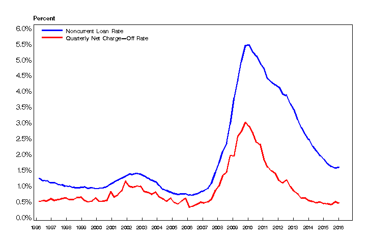
The historical US series illustrates this difference. It is not valid to infer a common denominator or annual horizon simply because both lines are percentages. The noncurrent series is a point-in-time stock ratio, whereas the displayed net-charge-off series is measured over a quarter using the source's convention. Timing and definitions must be checked before comparing their heights or using either as an estimate of prospective .
What historical lending-rate data show
The Swiss descriptive evidence below groups loans by size and product. The smallest displayed size class covers CHF 50,000–100,000 and the largest exceeds CHF 1 million; the intermediate classes are retained under their original labels because their precise cutoffs are not specified in this extract. Interest-rate columns are annual percentages. The observation count and share refer to the corresponding product's sample, not to the overall Swiss loan stock.
| Product | Size class | N | Sample share (%) | Mean (%) | Min (%) | 25th percentile (%) | Median (%) | 75th percentile (%) | Max (%) |
|---|---|---|---|---|---|---|---|---|---|
| Overdraft | 1 | 47,985 | 48.20 | 5.30 | 0.00 | 4.50 | 5.25 | 6.00 | 10.00 |
| Overdraft | 2 | 39,060 | 39.23 | 5.36 | 0.01 | 4.70 | 5.50 | 6.00 | 10.00 |
| Overdraft | 3 | 6,165 | 6.19 | 5.17 | 0.25 | 4.50 | 5.25 | 5.75 | 9.95 |
| Overdraft | 4 | 6,350 | 6.38 | 4.89 | 0.00 | 4.25 | 5.00 | 5.75 | 9.95 |
| Mortgage | 1 | 28,802 | 16.63 | 3.22 | 0.00 | 2.75 | 3.25 | 3.70 | 8.75 |
| Mortgage | 2 | 95,191 | 54.96 | 3.08 | 0.28 | 2.70 | 3.00 | 3.50 | 8.75 |
| Mortgage | 3 | 25,960 | 14.99 | 3.06 | 0.43 | 2.63 | 3.13 | 3.50 | 7.50 |
| Mortgage | 4 | 23,233 | 13.42 | 2.99 | 0.42 | 2.58 | 3.13 | 3.50 | 7.50 |
| Investment loan | 1 | 3,713 | 4.07 | 3.25 | 0.37 | 2.10 | 3.25 | 4.16 | 10.00 |
| Investment loan | 2 | 26,601 | 29.15 | 3.01 | 0.22 | 1.80 | 3.00 | 4.00 | 10.00 |
| Investment loan | 3 | 17,869 | 19.58 | 2.54 | 0.16 | 1.25 | 2.55 | 3.54 | 10.00 |
| Investment loan | 4 | 43,063 | 47.19 | 2.23 | 0.12 | 1.00 | 2.05 | 3.25 | 9.77 |
Mean investment-loan rates decline from 3.25% in class 1 to 2.23% in class 4, consistent with lower costs per franc for larger loans. The pattern is not strictly monotonic for every product, and it is not a controlled estimate of the causal effect of size. Borrower risk, collateral, maturity, bargaining and contract type also differ across groups. The minimum and maximum columns show that a class mean can conceal substantial dispersion.
| Product | Risk class | N | Sample share (%) | Mean (%) | Min (%) | 25th percentile (%) | Median (%) | 75th percentile (%) | Max (%) |
|---|---|---|---|---|---|---|---|---|---|
| Overdraft | 1 | 2,002 | 2.01 | 5.13 | 0.25 | 4.25 | 5.50 | 5.75 | 9.50 |
| Overdraft | 2 | 5,544 | 5.57 | 5.38 | 0.00 | 4.75 | 5.55 | 5.88 | 9.95 |
| Overdraft | 3 | 25,721 | 25.83 | 5.52 | 0.01 | 5.00 | 5.60 | 6.00 | 9.95 |
| Overdraft | 4 | 41,383 | 41.57 | 5.24 | 0.00 | 4.50 | 5.25 | 6.00 | 10.00 |
| Overdraft | 5 | 13,729 | 13.79 | 5.37 | 0.85 | 4.50 | 5.25 | 6.00 | 10.00 |
| Mortgage | 1 | 2,240 | 1.29 | 3.10 | 0.65 | 2.75 | 3.13 | 3.56 | 6.00 |
| Mortgage | 2 | 7,193 | 4.15 | 2.95 | 0.44 | 2.50 | 3.00 | 3.50 | 6.75 |
| Mortgage | 3 | 29,874 | 17.25 | 3.01 | 0.42 | 2.60 | 3.00 | 3.50 | 7.13 |
| Mortgage | 4 | 73,220 | 42.28 | 2.95 | 0.28 | 2.50 | 2.88 | 3.50 | 7.63 |
| Mortgage | 5 | 20,137 | 11.63 | 3.25 | 0.00 | 2.75 | 3.25 | 3.75 | 8.75 |
| Investment loan | 1 | 3,819 | 4.19 | 2.24 | 0.23 | 1.10 | 2.00 | 3.30 | 5.83 |
| Investment loan | 2 | 4,229 | 4.63 | 2.11 | 0.28 | 0.84 | 1.95 | 3.28 | 5.80 |
| Investment loan | 3 | 17,837 | 19.55 | 2.20 | 0.22 | 1.00 | 2.07 | 3.20 | 6.90 |
| Investment loan | 4 | 42,006 | 46.04 | 2.56 | 0.12 | 1.20 | 2.50 | 3.60 | 9.34 |
| Investment loan | 5 | 14,572 | 15.97 | 2.90 | 0.32 | 1.45 | 2.80 | 4.00 | 10.00 |
Class 1 denotes expected loss below 0.05% of exposure and class 5 expected loss above 2.6%; the intermediate class boundaries are not supplied here. Counts and percentages need not cover every observation in the size table, because an observation may lack a risk classification. In investment lending, the mean increases from 2.24% in class 1 to 2.90% in class 5, but the middle groups and the other products show why a raw average is not an exact pricing equation. Contract rates and expected losses can also be measured at different times.
Historical Swiss descriptive tables attributed to Cecchin (2011). Values are reproduced as historical observations, with the original class labels and the cutoffs actually provided; no unreported class boundaries or observation-level data have been inferred.
Debt funding, equity and a complete pricing calculation
Debt and equity supply funds in different ways. Depositors and other creditors have contractual claims; shareholders absorb residual losses and require compensation for that risk. A bank can allocate more equity capital to riskier exposures even though individual deposits and equity shares are not physically earmarked for particular loans. The allocation is a management representation of the loss-absorbing resources needed to support the asset, influenced by economic risk and regulatory constraints.
It is not valid to hold the required equity return fixed and conclude that reducing equity always creates a free saving. More leverage usually makes the remaining equity riskier, which can increase its required return. The cost of debt, distress costs, tax effects and constraints can also change. Similarly, expected loss should not be counted once as a loss allowance and again as an identical extra capital cost without explaining the convention.
Consider a EUR 1 million one-year loan with operating costs of EUR 5,000, and . The assigned funding is 90% deposits at 2% and 10% equity requiring 10%. Operating cost is 50 basis points, expected loss is 80 basis points and the weighted funding charge is . The additive required rate is therefore:
The corresponding annual revenue is EUR 41,000: EUR 5,000 for operations, EUR 8,000 for expected losses, EUR 18,000 for deposit interest and EUR 10,000 for the return on allocated equity. The last item is an economic required return, not an interest expense payable to shareholders in the profit-and-loss statement.
An exact cash-flow version illustrates why assumptions matter. Suppose the loan pays principal and its full coupon only if it survives to year-end, and a default instead returns at year-end with no coupon. Let and . Expected receipts must equal , giving:
Under these additional assumptions, the rate is , rather than 4.1%. The difference compensates for the coupon lost in default. Both calculations are understandable once their conventions are explicit; mixing the additive revenue convention with the terminal-default model silently produces an inconsistency.
Worked application: loan pricing and the bank's full income statement
Change the inputs to a EUR 1 million loan with EUR 5,000 operating cost, , , 90% deposit funding at 1% and 10% equity requiring 10%. Under the additive convention, the required rate is . Now suppose the bank starts the year with EUR 80 million of such loans and EUR 20 million of liquidity earning no interest. It is funded with EUR 90 million of deposits and EUR 10 million of equity, has no other revenue or costs and ignores taxes.
| Assets | Amount | Liabilities and equity | Amount |
|---|---|---|---|
| Liquidity | 20.00 | Deposits | 90.00 |
| Loans | 80.00 | Equity | 10.00 |
| Total assets | 100.00 | Total liabilities and equity | 100.00 |
| Item | Calculation | Amount |
|---|---|---|
| Interest income | 80 × 4.4% | 3.52 |
| Deposit interest expense | 90 × 1% | −0.90 |
| Net interest income | 3.52 − 0.90 | 2.62 |
| Loan-loss expense | 80 × 2% × 100% | −1.60 |
| Non-interest income | Assumed absent | 0.00 |
| Trading income | Assumed absent | 0.00 |
| Salary and administrative cost | 80 loans × EUR 5,000 | −0.40 |
| Profit before tax | 2.62 − 1.60 − 0.40 | 0.62 |
Profit of EUR 0.62 million on EUR 10 million of equity implies a pretax return of 6.2%, below the 10% required return. This is not a failure of arithmetic: the 4.4% rate was calibrated to the funding and equity allocated to the loan itself, while one-fifth of the bank's assets earns nothing. The loans support EUR 8 million of allocated equity and generate the corresponding EUR 0.8 million before the funding cost of the liquidity buffer. The buffer uses EUR 18 million of deposits costing EUR 0.18 million and EUR 2 million of equity, giving actual accounting profit of EUR 0.62 million and an economic shortfall of EUR 0.38 million relative to the whole bank's EUR 1 million target.
To achieve the whole-bank pretax target under the same additive assumptions, total loan revenue would have to cover million euros, requiring on the loans. Liquidity is useful despite its opportunity cost, so this result is a reason to price and allocate that cost explicitly, not to assume the bank should hold none. Under the alternative terminal-default convention, the original 4.4% quote would instead need to be for the isolated loan; its income statement would also need to use expected collected coupons consistently.
Borrower participation under limited liability
Now consider 2,000 applicants who each need an indivisible investment of 100 monetary units. Half are lower-risk borrowers with success probability and project proceeds on success. Half are higher-risk borrowers with and . Both receive zero on failure. Applicants know their types; the bank cannot distinguish them and cannot use a signal or collateral in this model. The bank has at most 100,000 units of funds, enough for 1,000 loans, and the risk-free funding rate is .
At the contractual lending rate , debt due is . A risk-neutral borrower of type receives the limited-liability payoff in the success state and zero otherwise. Expected private surplus is therefore:
The participation rule here requires strictly positive surplus. Lower-risk applicants borrow only for , while higher-risk applicants borrow for . At the threshold a borrower is indifferent and, by convention, does not apply. While both types participate, their expected surpluses are and . These linear expressions should not be extrapolated into negative private payoffs after limited liability binds; the borrower instead declines the loan.
The safer type has the higher expected project output, , compared with . Nevertheless, the riskier type is willing to accept a higher promised interest rate because its success-state upside is larger and repayment is required less often. A willingness to pay more is therefore not sufficient evidence that an applicant is a better credit risk.
Expected lender receipts and the correct supply intervals
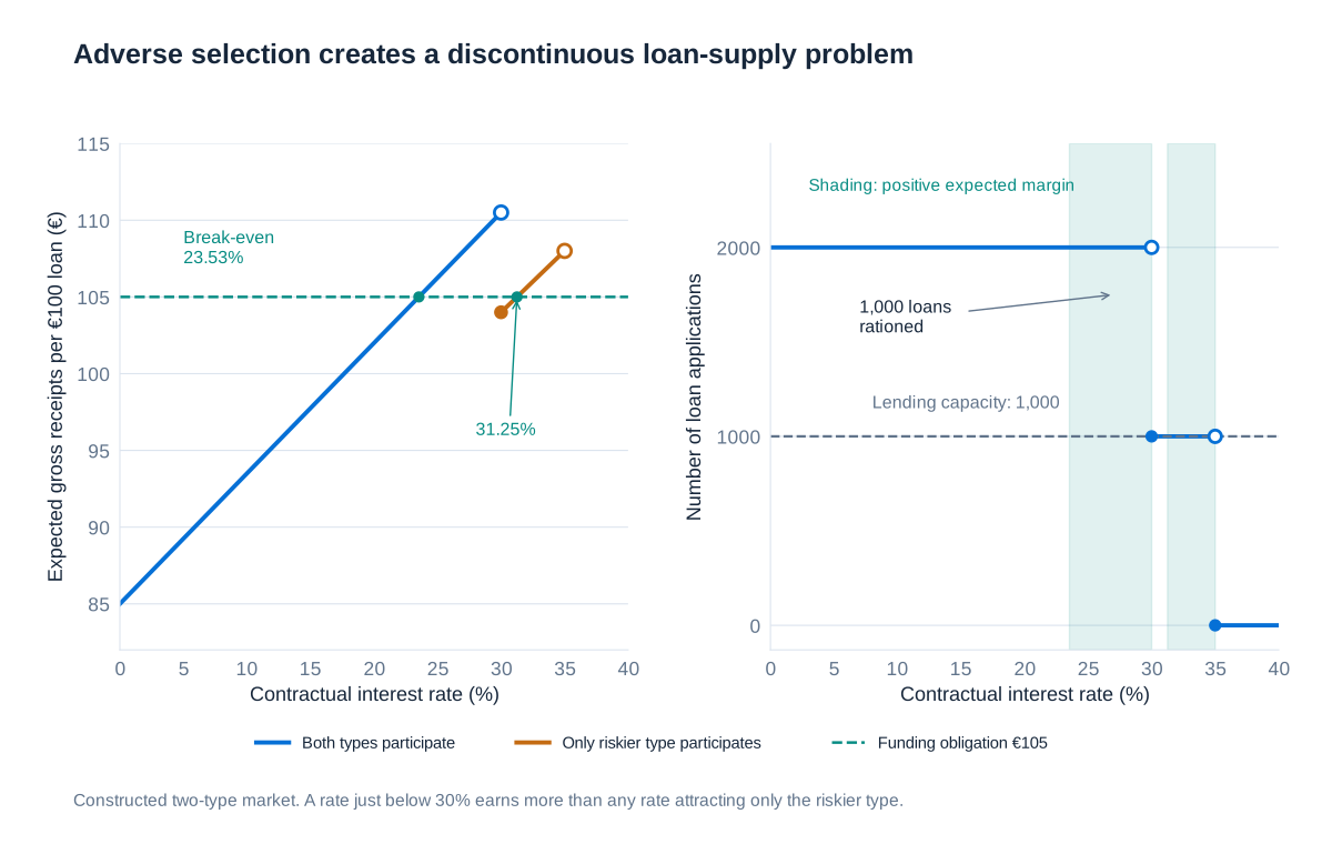
Let denote the bank's expected gross repayment per loan of 100. When both groups apply, average success probability is . At 30% the safe borrowers leave, reducing this probability to 0.8. Consequently:
At rates of 35% or more there are no applicants under the strict-participation rule, so the bank makes no loans. Gross repayments are not profits: the bank must pay 105 per funded loan to cover principal and the 5% funding obligation. Expected net profit is . In particular, the break-even rate while both types apply is , not 23.52% exactly.
| Contract rate | Applicants | Mean success probability | Gross receipts | Profit after funding cost |
|---|---|---|---|---|
| 0% | 2000 | 0.85 | 85.0000 | -20.0000 |
| 5% | 2000 | 0.85 | 89.2500 | -15.7500 |
| 10% | 2000 | 0.85 | 93.5000 | -11.5000 |
| 15% | 2000 | 0.85 | 97.7500 | -7.2500 |
| 20% | 2000 | 0.85 | 102.0000 | -3.0000 |
| 23.5294…% | 2000 | 0.85 | 105.0000 | 0.0000 |
| 25% | 2000 | 0.85 | 106.2500 | 1.2500 |
| 29.99% | 2000 | 0.85 | 110.4915 | 5.4915 |
| 30% | 1000 | 0.80 | 104.0000 | -1.0000 |
| 31% | 1000 | 0.80 | 104.8000 | -0.2000 |
| 31.25% | 1000 | 0.80 | 105.0000 | 0.0000 |
| 34.99% | 1000 | 0.80 | 107.9920 | 2.9920 |
| 35% | 0 | No applicants | No loan | Not applicable |
| 40% | 0 | No applicants | No loan | Not applicable |
The first profitable interval is above approximately 23.5294% and below 30%. Immediately at 30%, gross receipts fall from nearly 110.5 to 104, so lending becomes unprofitable again. The high-risk-only pool breaks even at , and is profitable between 31.25% and 35%. At either break-even boundary the bank is indifferent; an explicit tie rule would determine how much it lends. A graph showing capacity of 1,000 loans at every rate above the first break-even threshold would therefore be incorrect.
Expected receipts rise toward 110.5 just below 30% and toward only 108 just below 35%. With a smallest rate increment of one basis point, the preferred offer is 29.99%, giving receipts of 110.4915 and profit of 5.4915 per loan. If rates were continuous and borrowers refused exactly at zero surplus, “just below 30%” would describe a supremum rather than an attained exact optimum. Stating the rate increment or participation convention removes this minor mathematical ambiguity.
Why the bank rations credit instead of raising the rate
At 29.99%, all 2,000 applicants want loans, but the bank can finance only 1,000. With no additional way to distinguish applicants, it grants 1,000 loans and rejects 1,000 interested borrowers. Raising the rate to reduce demand changes the composition of applicants and lowers the bank's maximum expected receipts. Quantity rationing is therefore compatible with profit maximisation; the bank need not be subject to an externally imposed interest-rate ceiling.
An outright refusal to an applicant who accepts the offered terms is called type 1 rationing here. Granting less than the requested amount is type 2 rationing. If investment were perfectly divisible and payoffs scaled proportionally, the bank could distribute 50 units to each applicant rather than 100 to half of them. That alternative requires divisible productive opportunities; providing half the financing for an indivisible project may make the whole project impossible.
The finite funding capacity is part of this example. The wider Stiglitz–Weiss insight is that information and incentive effects can prevent the interest rate from clearing the credit market, even though some rejected applicants would accept the price. Rejection alone does not prove this mechanism: a borrower can also be denied because the project is unviable, legal conditions are unmet or the bank cannot assess repayment. Nor is every borrower who declines an expensive offer quantity-rationed. A precise analysis separates demand at the offered terms from the supply decision.
Alternatives include better screening, monitoring, collateral, guarantees, shorter maturities or relationships that reveal information. Each has costs and may change which customers can borrow. A collateral requirement can screen risk but exclude asset-poor applicants; more screening can improve decisions but be too costly for a small loan. The existence of a remedy in theory does not mean that credit rationing vanishes in practice.
Three worked variations on the rationing model
Keep 2,000 applicants, a loan size of 100, equal type shares and capacity for 1,000 loans, but set the funding rate to zero. In each variation, compare the bank's expected receipts near the participation cutoffs rather than assume that adverse selection always implies rationing. Rates written as a cutoff below mean the limit from below, or the closest feasible lower quote if the bank uses a discrete rate grid.
| Variation | Type I: success / failure proceeds and probability | Type II: success / failure proceeds and probability | Receipts with both types near the lower cutoff | Receipts with the remaining type near its cutoff | Preferred outcome |
|---|---|---|---|---|---|
| A | 130 / 0; p = 0.9 | 120 / 0; p = 0.8 | 0.85 × 120 = 102 near 20% | 0.9 × 130 = 117 near 30% | Only type I borrows; no quantity rationing |
| B | 130 / 80; p = 0.9 | 135 / 0; p = 0.8 | 0.5(0.9 × 130 + 0.1 × 80) + 0.5(0.8 × 130) = 114.5 near 30% | 0.8 × 135 = 108 near 35% | Both types apply; 1,000 applicants rejected |
| C | 130 / 0; p = 0.9 | 150 / 0; p = 0.8 | 0.85 × 130 = 110.5 near 30% | 0.8 × 150 = 120 near 50% | Only type II borrows; no quantity rationing |
In variation A, the safer borrower also has the higher success-state return. The riskier type exits around 20%, so an increase in the rate improves the applicant pool. Charging just below 30% attracts exactly the 1,000 safer applicants and produces receipts close to 117, more than the 102 available just below 20%. Every applicant willing to borrow at the selected rate receives a loan, even though the other type declines to apply. This is price selection rather than quantity rationing.
In variation B, the lower-risk project produces 80 even in its unsuccessful state. Near the 30% cutoff, the bank's expected receipt from this type is ; from the higher-risk type it is . Their average is 114.5. If the safe borrowers withdraw and the bank raises the rate toward 35%, receipts reach only 108. It prefers the lower rate and rationing. The 80-unit recovery must be included in bank receipts; it is not a payment retained by the borrower because the debt exceeds 80 in this region.
In variation C, adverse selection still occurs at 30%, but the riskier project's success-state proceeds are large enough to support a rate near 50%. Receipts of 120 exceed 110.5, so the bank chooses the high-risk-only pool and fills its 1,000-loan capacity without rejecting any willing applicant. Adverse selection is thus a mechanism that can cause rationing, not a sufficient condition for it. The lender must compare the entire expected-receipts schedule.
Empirical evidence on requested and granted credit
To study rationing, one needs to observe what borrowers requested as well as what banks granted. A database containing only completed loans cannot directly show whether a firm wanted more. Kirschenmann's study uses roughly 98,000 matched applications and contracts for micro and small businesses at a Bulgarian bank during 2003–2007. The firms had mean assets around EUR 35,000 and mean age around eight years; loans averaged approximately EUR 5,000 with maturity around 28 months. Firms appear in sequences of one to ten loans. Interest and collateral terms followed the bank's fixed contractual framework, which makes the approved amount an especially relevant adjustment margin.
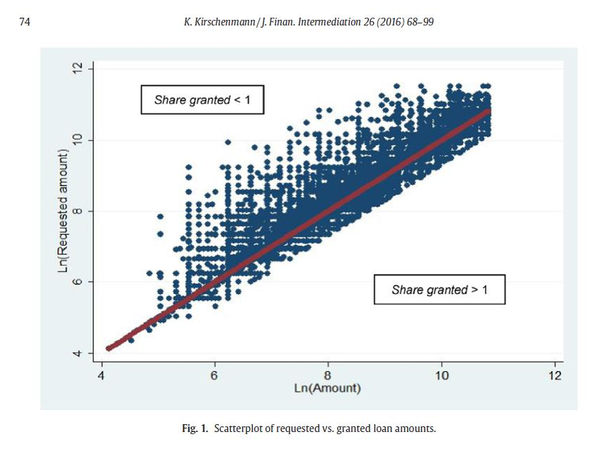
In the scatter, the horizontal axis is the logarithm of the granted amount and the vertical axis the logarithm of the requested amount. The 45-degree line means request equals grant. A point above it means the request exceeds the grant, so the granted share is below one. Logarithms show proportional differences; the vertical gap is the logarithm of the requested-to-granted ratio, not an amount in euros. Observations below the line have granted amounts exceeding the recorded request and should not be mistaken for rationing.
| Comparison | First loans: share granted | Later loans: share granted | Difference-in-differences |
|---|---|---|---|
| Initially young firms | 0.856***; SE 0.002; N = 11,428 | 0.938***; SE 0.003; N = 6,404 | Not separately reported |
| Initially old firms | 0.905***; SE 0.001; N = 41,933 | 0.954***; SE 0.001; N = 37,129 | Not separately reported |
| Young minus old | −0.050***; SE 0.002; N = 53,361 | −0.016***; SE 0.003; N = 43,533 | −0.033***; SE 0.004; N = 96,894 |
SE denotes standard error and N the number of observations. Three stars indicate significance at the 1% level in the reported table; the original convention also uses two stars for 5% and one for 10%. The first-loan gap means young firms receive about five percentage points less of their requested credit than old firms. The gap is narrower for later loans. The reported difference-in-differences uses the first-loan gap minus the later-loan gap, explaining its negative sign. Its value and the differences need not equal subtraction of the rounded displayed means exactly.
The wider evidence finds more rationing for young, small and previously unbanked firms and a reduction over repeated borrowing. This is consistent with information accumulation, but descriptive associations do not by themselves identify a single causal explanation. Continuing borrowers are a selected group; collateral, risk, profitability and requested amounts may change with experience. The result supports the importance of opacity and relationship history without proving that every reduction in rationing is caused by private information alone.
Karolin Kirschenmann (2016), Credit rationing in small firm-bank relationships, Journal of Financial Intermediation 26, 68–99. Table values and the scatter refer to this historical sample, not to all firms or present-day Bulgarian lending.
Two banks and the winner's curse of uninformed lending
Suppose half the applicants always repay and half never repay. Bank 1 has perfect screening and can distinguish the types; Bank 2 cannot. Each bank simultaneously chooses whether to offer a loan and its rate, capped at 200%, and a repayable borrower prefers a lower rate. For the following calculation, normalise principal to one and set the funding cost to zero. Screening costs, capacity constraints and borrower surplus limits are ignored. Tie-breaking and how non-repaying applicants choose between offers matter for a full game-theoretic solution.
Without a competitor, the uninformed bank would break even at 100% interest because . It might therefore believe that offering 100% to everyone is safe. But the relevant repayment probability is conditional on winning the customer. Bank 1 can offer 99% only to good borrowers and decline bad borrowers. Good customers choose Bank 1; Bank 2 is left with the non-repaying group and receives zero. The applicant pool before competition is not the pool that accepts the uninformed bank's offer afterward.
The offer “Bank 1 lends to good applicants at 99%; Bank 2 stays out” is useful for understanding entry deterrence. To win good customers by undercutting 99%, Bank 2 must quote a rate at which even the original half-good pool is loss-making. A higher offer loses the good borrowers to the informed bank. Bank 1 can earn an information rent even though Bank 2 is potentially available as a competitor.
However, that offer pair is not a Nash equilibrium of the simultaneous game as stated. If Bank 2 has already chosen no offer and that strategy is held fixed, Bank 1 can profitably raise its rate to the permitted cap for the good borrowers. Conversely, sufficiently high pricing by Bank 1 would invite a profitable undercutting offer from Bank 2 when the original pool includes enough good customers. A complete equilibrium analysis needs explicit borrower payoffs and tie rules and may require mixed strategies. The 99% example is an explanation of the information problem, not a solved equilibrium that should be presented as one.
The economically durable conclusions are that information has value, that avoiding a market can be rational for a poorly informed lender, and that a bank's profit depends on its information advantage relative to competitors. Knowing what other lenders know can be as important as knowing the unconditional average default rate. This is the credit-market version of a winner's curse: winning business can itself be bad news when a better-informed competitor declined it.
How relationship banking changes information and incentives
Relationship banking develops when repeated interactions provide the lender with private information about a borrower. Repeated loans reveal repayment behaviour and the reliability of earlier forecasts. Cross-selling, such as providing the operating account as well as a loan, reveals incoming receipts, payment obligations and changes in liquidity. Such information can be “soft”: knowledge of management competence or customer stability may be valuable even when it cannot be reduced to a public, verifiable score.
Information accumulation can reduce adverse selection, while the prospect of future access to credit can reduce moral hazard. An entrepreneur may work harder and avoid excessive risk when poor behaviour threatens a continuing valuable relationship. The bank may also distinguish a temporary cash-flow shock from a deteriorating business more effectively than a new outside lender. These benefits are strongest when monitoring is credible and continuation depends on repayment and performance rather than unconditional support.
| Country | Firms (N) | Mean relationships | Median | Maximum | One bank (%) | Two banks (%) | Three to seven (%) | More than seven (%) |
|---|---|---|---|---|---|---|---|---|
| Italy | 64 | 15.2 | 12 | 70 | 3.1 | 3.1 | 23.4 | 70.3 |
| Portugal | 39 | 11.5 | 10 | 40 | 5.1 | 2.6 | 30.8 | 61.5 |
| France | 24 | 11.3 | 9 | 50 | 4.2 | 4.2 | 33.3 | 58.3 |
| Belgium | 8 | 11.1 | 7 | 30 | 0.0 | 25.0 | 25.0 | 50.0 |
| Spain | 68 | 9.7 | 7 | 60 | 1.5 | 7.4 | 44.1 | 47.1 |
| Germany | 63 | 8.1 | 5 | 29 | 15.9 | 7.9 | 39.7 | 36.5 |
| Greece | 37 | 7.4 | 6 | 19 | 0.0 | 8.1 | 51.4 | 40.5 |
| Austria | 36 | 5.2 | 3 | 22 | 19.4 | 13.9 | 44.4 | 22.2 |
| Luxembourg | 7 | 5.0 | 4 | 18 | 28.6 | 0.0 | 57.1 | 14.3 |
| Czech Republic | 58 | 4.7 | 4 | 14 | 3.4 | 10.3 | 70.7 | 15.5 |
| Switzerland | 36 | 3.6 | 2 | 40 | 41.7 | 19.4 | 30.6 | 8.3 |
The historical corporate comparison shows that relationship lending need not mean having only one bank. In the displayed Italian sample, the median firm had 12 relationships; in the Swiss sample it had two. The distinction between a mean and a median matters because a few firms with many banks can raise the mean substantially. The small country samples and historical setting limit generalisation, and the percentages can differ slightly from 100 because of rounding. Maintaining several banks can diversify funding risk and bargaining options, while still allowing one bank to be the principal relationship lender.
Corporate relationship data: Ongena and Smith (2000), historical cross-country sample. The table reproduces the countries and variables available in the supplied excerpt; it is not a current census of European firms.
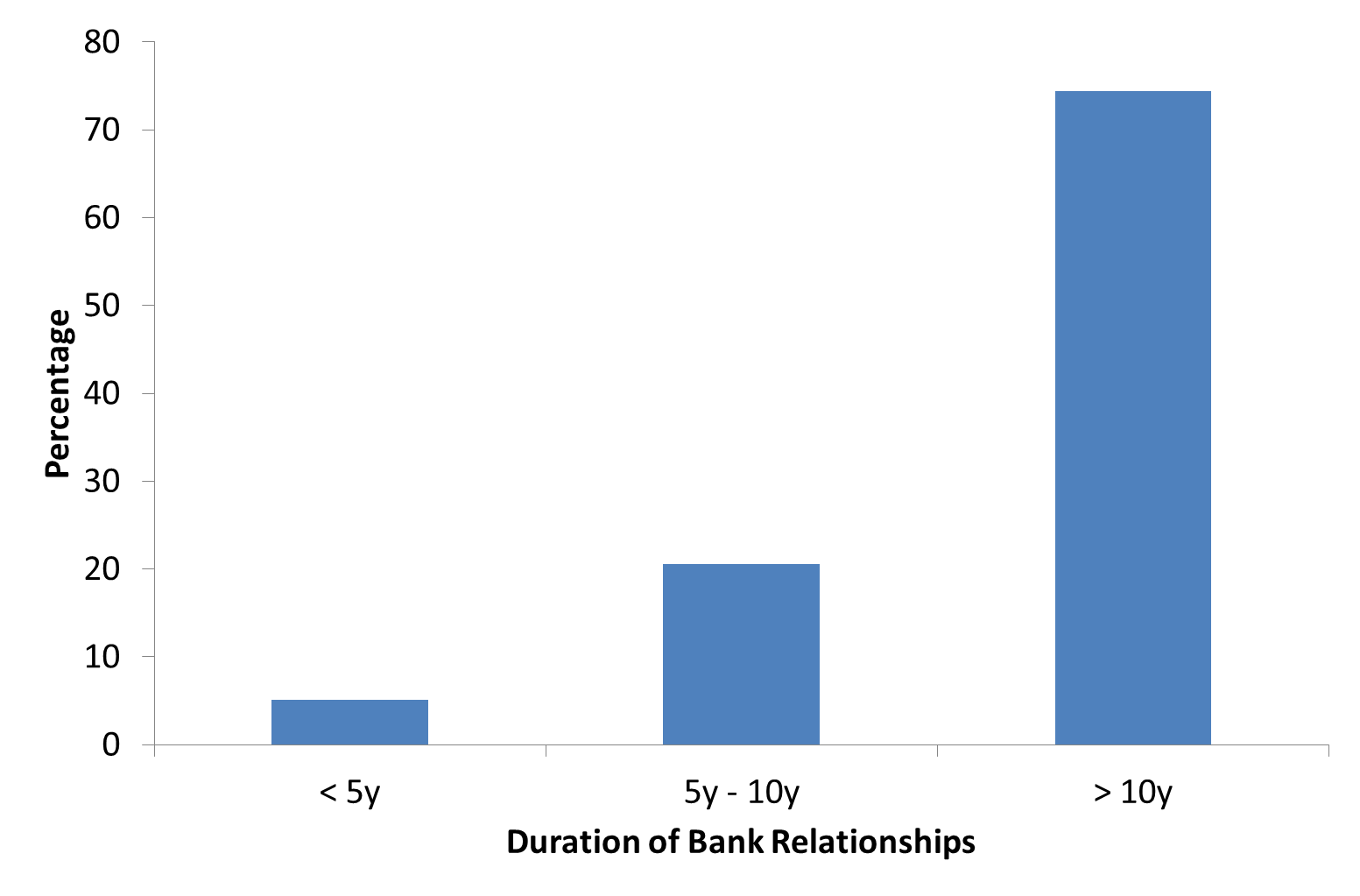
Household relationships can also persist for many years. The historical sample in the duration chart contains 2,644 bank relationships belonging to 1,456 households, so the observational unit is a relationship rather than a unique person. Most relationships in the chart lasted more than ten years. The difference between the number of households and relationships also shows that households can use several banks at once.
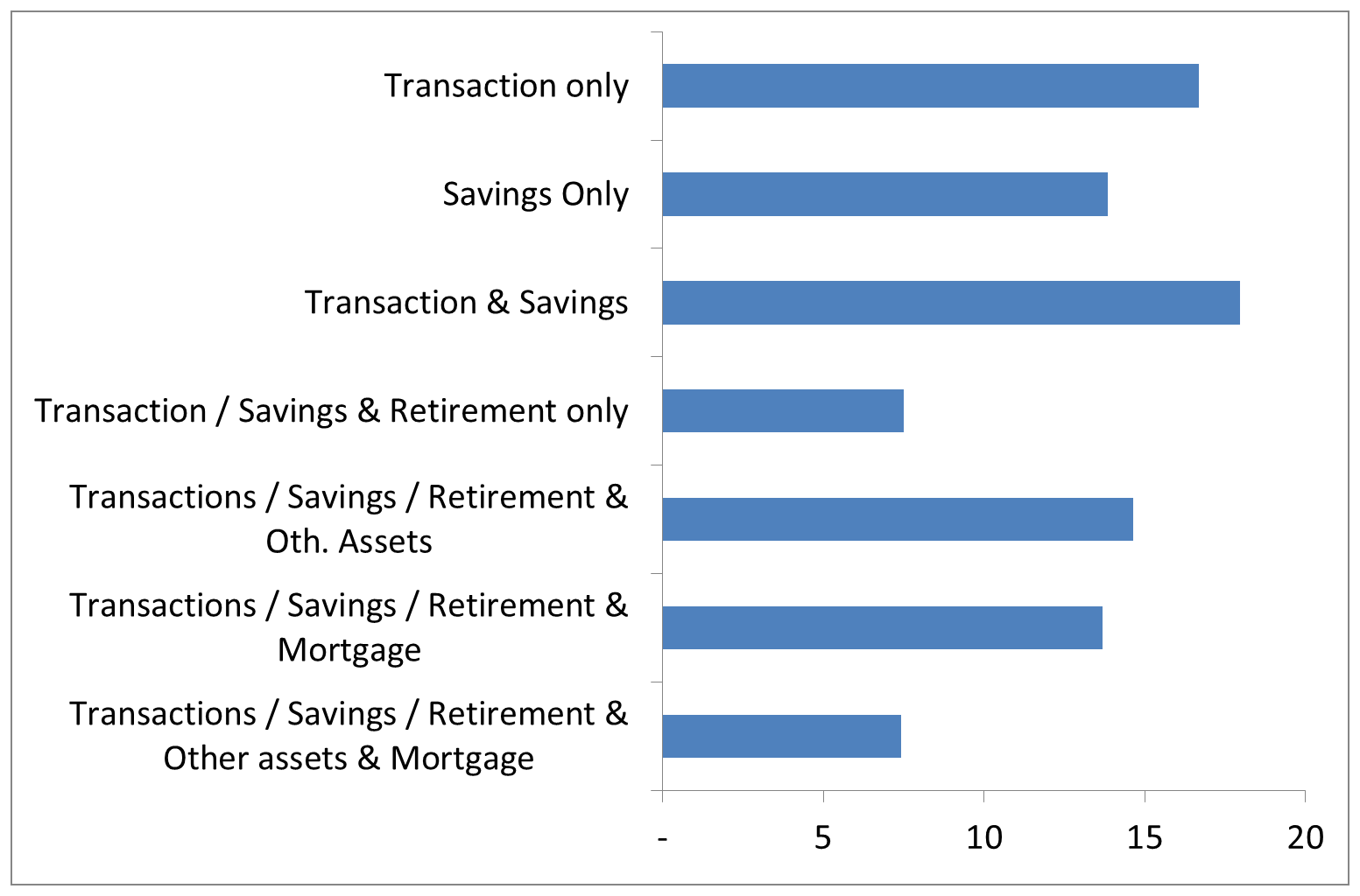
The product-scope chart describes combinations of transactions, savings, retirement products, other assets and mortgages. A broad relationship can supply the bank with information across several financial activities, while also increasing the customer's switching effort. The categories describe product bundles, not an ordering from “good” to “bad” customers. Their historical proportions must not be treated as individual borrowers' credit scores or evidence that cross-selling automatically improves welfare.
Historical household relationship charts attributed to Brown and Hoffmann (2016 for duration; 2013 for product scope), using 2,644 relationships of 1,456 households. Approximate visual heights are not converted into invented exact observations.
The benefits and costs of an informed incumbent
A relationship can improve access to credit, reduce repeated screening costs and allow useful flexibility during temporary difficulty. But private information also creates a potential hold-up problem: outside banks may fear that a borrower seeking to switch is one the incumbent knows to be weak. The incumbent can then gain pricing power because competitors cannot reproduce its information cheaply. The two-bank example explains why more nominal competitors do not guarantee equal information or aggressive price competition for every customer.
Other risks include dependence on one bank's funding health, conflicts across the bank's advisory and lending roles, and excessive forbearance when a lender protects an existing exposure by advancing more funds to a weak borrower. Multiple relationships, transferable information, credit registries and transparent financial reporting can limit these costs, but they can also reduce each bank's incentive to invest in proprietary monitoring. The appropriate structure balances information production, competition and continuity rather than treating either transactional lending or relationship banking as universally superior.
The main connection is that pricing, quantities and information are jointly determined. A higher coupon may compensate for a given risk, yet also change that risk through selection and incentives. A longer relationship may improve screening, yet create market power. Sound lending therefore assesses the entire contract and customer relationship: expected cash flows, operating and funding costs, capital, collateral, information and the consequences of competing offers.