
9. Earnings at Risk and Cash Flow at Risk
Three different objects of risk management
A financial position has a market value, produces accounting results and generates cash payments. These three descriptions are related, but they are not interchangeable. A bond can lose market value without changing its contractual coupon; a derivative can generate an immediate collateral payment while the benefit of the exposure it hedges will arrive years later. A useful risk analysis therefore specifies what must remain stable, for whom, and over what horizon.
Value at Risk concerns a distribution of economic or market-value losses. Earnings at Risk concerns a distribution of reported earnings, after applying the relevant recognition and measurement rules. Cash Flow at Risk concerns a distribution of cash receipts, payments or their net amount. Each requires a horizon, a confidence level and a precise boundary: consolidated earnings differ from one subsidiary’s earnings, and cash available in one currency or legal entity may not be available elsewhere.
Let denote earnings over horizon , net cash flow over that horizon, and the lower quantile of a random variable . One useful shortfall convention, adopted here, measures the distance from specified benchmarks and . At confidence level , define:
The benchmarks might be expected results or an approved budget; the choice must be disclosed. These measures are currency amounts, not probabilities. An EaR of €6 million does not mean that earnings will be negative by €6 million: it means that the selected lower-tail result is €6 million below the stated benchmark. Some organisations instead report the lower-tail earnings or cash-flow level itself. Reporting both the level and the shortfall prevents this terminology from obscuring the result.
Objectives, earnings expectations and managerial incentives
Different decision makers reasonably emphasise different outcomes. A bank manager may prioritise stable reported profits, a fund manager the value available to investors who redeem, and a household predictable mortgage instalments. A pension investor with known nominal payments may accept fluctuations in asset prices to secure the required future receipts. The correct objective depends on liabilities and withdrawal needs, not solely on the instrument’s standalone volatility.
The importance attached to recurring earnings is visible in public discussions of bank strategy. Morgan Stanley’s emphasis on more stable revenues in January 2023 illustrates the attraction of predictable business income. Debates about Josef Ackermann’s 25% return target at Deutsche Bank illustrate a different concern: a high return target can encourage leverage or risk taking if its risk cost is ignored. Stable reported earnings and a high reported return are not sufficient descriptions of a sound business model.
Market reactions also depend on expectations beyond the current earnings number. A company may beat analysts’ estimates while its share price falls because future guidance disappoints, discount rates rise or the result was already anticipated. Commentary on the second quarter of 2023 described precisely this combination. It does not establish that positive surprises are generally unwelcome. The quality, persistence and information content of earnings matter alongside their level.
Burgstahler and Eames (2006) examine how managers avoid negative earnings surprises. Their evidence links small non-negative surprises both to management of reported earnings and to management of analysts’ expectations, with roles for operating cash flows and discretionary accruals. For risk management, this raises a governance problem: an incentive to achieve a reported target can favour accounting outcomes over economic resilience. An instrument that smooths one reported number may increase financing needs elsewhere.
Choices can therefore involve genuine trade-offs. If strategy A has lower market-value risk but higher cash-flow risk than strategy B, neither dominates without information about the investor’s constraints. If A reduces all relevant risks for the same expected return and cost, B is harder to justify. A practical decision compares the full set of outcomes, including transaction costs, liquidity needs and the consequences of the adverse scenarios.
How accounting translates economic changes into earnings
Accounting determines when an economic change reaches profit or loss. Under IFRS 9, the classification of a debt financial asset depends principally on its business model and the characteristics of its contractual cash flows. The SPPI test asks whether those cash flows are solely payments of principal and interest on the principal outstanding. A prudential label such as “banking book” does not by itself establish the accounting category.
| Business model | Contractual cash-flow condition | Usual measurement category |
|---|---|---|
| Hold assets to collect contractual cash flows | SPPI condition satisfied | Amortised cost |
| Collect contractual cash flows and sell assets | SPPI condition satisfied | Fair value through other comprehensive income (FVOCI) |
| Other business models, or a failed SPPI condition | The preceding combinations do not apply | Fair value through profit or loss (FVTPL) |
The fair-value option can also be relevant when its conditions are met, including elimination or significant reduction of an accounting mismatch. Equity investments require separate classification considerations. The table is therefore a framework for ordinary debt assets, not a universal decision rule for every financial instrument.
Amortised cost does not mean that the balance-sheet amount remains permanently equal to purchase price. Effective-interest accruals, amortisation of premiums or discounts, repayments and expected credit losses can change the amount and the earnings recognised. What is generally absent is immediate recognition in profit or loss of every market-price movement caused solely by changes in market yields. For an FVTPL instrument, those valuation changes normally affect current earnings.
Other comprehensive income, or OCI, is outside the current profit-or-loss subtotal but remains part of comprehensive income and equity. A valuation movement reported in OCI has not disappeared economically. It can still affect capital, contractual constraints or the amount obtainable on sale. Risk managers must distinguish a stable profit-or-loss number from a stable balance sheet and from stable cash.
What hedge accounting changes
A derivative remains measured at fair value even when it participates in a qualifying hedge-accounting relationship. Hedge accounting changes the recognition of gains and losses to represent that relationship more faithfully. It requires an eligible relationship, documentation and satisfaction of the applicable effectiveness requirements; simply calling a transaction a hedge is insufficient.
The three main relationships have different accounting mechanics. In a fair-value hedge, changes in the hedging instrument and changes in the hedged item attributable to the designated risk generally enter profit or loss together. In a cash-flow hedge, the effective portion is initially recognised in OCI and is subsequently reclassified or incorporated into an asset’s carrying amount when the relevant rules require; ineffectiveness generally affects profit or loss. A hedge of a net investment in a foreign operation has an OCI treatment for its effective component associated with foreign-currency translation.
These distinctions explain why the statement “hedge losses go to OCI” is too broad. The accounting outcome depends on the designation and the underlying exposure. Moreover, no recognition rule cancels a derivative’s contractual settlement or collateral obligation. A hedge can improve the matching of reported earnings and still require substantial cash before the hedged transaction generates receipts.
Accounting sources: IFRS Foundation, IFRS 9 Financial Instruments, and the issued standard. Research reference: David Burgstahler and Michael Eames (2006), Management of Earnings and Analysts’ Forecasts to Achieve Zero and Small Positive Earnings Surprises.
One bond exposure, two financing and settlement patterns
Consider a hypothetical €100 long exposure to a very long-term bond with modified duration of 30 years. The exposure can be obtained by purchasing the bond or by taking an appropriately sized long position in a bond futures contract. Ignore basis changes and other differences initially. If the market yield rises by one percentage point, the first-order duration approximation is:
Here is the initial bond value, modified duration and the yield change expressed as a decimal. The 30% fall is an approximation; for such a large duration and yield shock, convexity can materially change the exact answer. This is a stress scenario, not a statistical VaR estimate unless a probability model and confidence level are supplied.
| Position and measurement | Economic value | Current earnings | Cash consequences after establishment |
|---|---|---|---|
| Purchased bond at amortised cost | Approximately €30 lower | No automatic €30 yield-driven fair-value loss; interest and impairment rules still apply | Contractual coupons continue if paid; a cash-funded holding has no futures variation margin |
| Purchased bond at FVTPL | Approximately €30 lower | Approximately €30 valuation loss in this simplified scenario | The valuation loss alone is not a cash payment; sale or secured financing can introduce cash effects |
| Long bond futures, without qualifying hedge accounting | Approximately €30 adverse change for matched exposure | Futures losses affect profit or loss | Variation margin produces cash payments as prices fall |
| Long bond futures in a qualifying hedge | The economic loss on the futures remains | Recognition depends on the designated hedge relationship | Collateral and settlement obligations remain payable |
The purchased bond requires the purchase price at inception. A futures position generally requires initial margin rather than payment of the full underlying value, but this smaller initial cash commitment is followed by potentially large variation-margin payments. Locating the futures in a particular management book does not remove these calls. If the purchased bond itself is financed through short-term borrowing or repo, its funding and collateral risks must also be added.
Thus similar interest-rate sensitivity can coexist with different EaR and CFaR. A statement that the directly purchased bond has “zero cash-flow risk” is defensible only within the narrow assumption of fixed contractual payments, no default, no optionality and no refinancing need. It is not a description of the investor’s entire balance sheet.
The perpetuity: stable income and unstable wealth
Suppose a 60-year-old retiree, Mr Rich, invests €10 million and wants a constant nominal income for an uncertain remaining lifetime. Assume a flat annual yield of 1% and an ideal default-free, non-callable perpetuity. A perpetuity pays the same amount at the end of every year forever. Its value is:
The yield is annual and expressed as a decimal; is euros per year and euros. Under these assumptions, the retiree receives €100,000 each year regardless of subsequent market yields. The investment meets the objective of constant nominal receipts without requiring a known date of death. It does not preserve purchasing power if prices rise, and real securities can introduce credit, call, tax and liquidity risks that the idealisation excludes.
| Market yield | Market value | Annual contractual income | Change from the initial €10 million value |
|---|---|---|---|
| 1% | €10,000,000 | €100,000 | €0 |
| 2% | €5,000,000 | €100,000 | −€5,000,000 |
| 5% | €2,000,000 | €100,000 | −€8,000,000 |
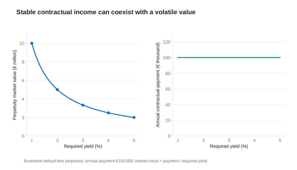
If the daughter inherits the security and immediately sells it after yields have risen to 5%, she receives €2 million. The same security is attractive to the father’s nominal-income objective and risky for the daughter’s eventual sale proceeds. The decline in market value reflects the lower attractiveness of the fixed coupon relative to newly available yields; it does not require any reduction in the promised coupon. A rise from 1% to 2% already halves the price, illustrating why percentage-point changes must be interpreted relative to the starting yield.
Fixed coupons, floating rates and the funding side
A floating-rate note resets its coupon periodically, for example every six months. A stylised coupon for period is , where is principal, the annual reference rate fixed for that period, the contractual annual spread and the year fraction. If the discount spread matches the contractual spread and credit and other conditions are unchanged, its ex-coupon value is approximately par at a reset date. Between resets, and when credit spreads change, its price can move.
The floating-rate investor therefore exchanges relatively stable interest-rate-related market value for variable future income. A fixed-rate investor makes the opposite exchange. A mortgage borrower who must meet instalments from a stable salary may value fixed nominal payments; a borrower expecting an early repayment may instead care about market-value changes and contractual termination charges. Neither preference is universal, and inflation changes the meaning of a “stable” nominal payment.
The same asset can also produce different earnings risk depending on the liabilities financing it. Suppose a bank’s deposit interest expense responds only weakly to market rates. Floating-rate assets then make net interest income sensitive to those rates, whereas fixed-rate assets can initially stabilise the margin. If deposit costs subsequently reprice rapidly, the conclusion may reverse. Deposit behaviour, maturity and customer options must be modelled rather than assumed permanently stable.
A fair-value portfolio assessed over the next quarter places considerable weight on price changes. An amortised-cost portfolio assessed over ten years places greater weight on interest margins, reinvestment and credit costs. The horizon and measurement basis explain much of the apparent disagreement over whether a fixed-rate bond is a high-risk or low-risk asset. A long-term liability with matching sensitivity can also offset the asset’s value risk at the portfolio level.
Building earnings and cash-flow distributions
A practical model starts with common economic scenarios and maps each scenario into both an income statement and a cash schedule. Sales volumes, selling prices, exchange rates, interest rates, credit losses and input costs influence earnings. Collection delays, inventory purchases, capital expenditure, debt maturities and derivative margin determine when cash moves. Depreciation reduces accounting earnings without a contemporaneous payment; a capital purchase can consume cash well before its expense is fully recognised.
Consider an explicitly hypothetical annual model with normally distributed earnings of mean €20 million and standard deviation €4 million, and normally distributed net cash flow of mean €15 million and standard deviation €6 million. Use each mean as its benchmark. At a one-sided 95% confidence level, the standard-normal lower quantile is approximately −1.645. The calculations, in millions of euros, are:
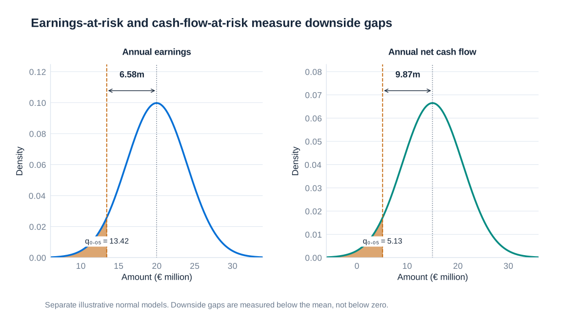
The example assumes separate marginal distributions and makes no claim about their correlation. The larger CFaR is consistent with cash being more sensitive to timing and financing shocks than earnings. The lower cash-flow quantile remains positive; the €9.87 million figure is a shortfall from the mean, not a €9.87 million cash loss. Normality is a teaching assumption and can miss asymmetric losses, defaults and discrete collateral triggers.
A terminal annual cash figure also cannot establish that every payment can be met during the year. A firm may finish December with positive cumulative cash after becoming unable to pay in June. Accordingly, cash-flow simulation should retain intermediate dates, currency needs, accessible reserves and committed funding. Stress scenarios complement quantiles by examining severe combinations that a fitted distribution may underrepresent.
Central-bank profits, gold and valuation reserves
Central banks illustrate why reported profit volatility cannot be read as a complete ranking of economic risk. The following historical figures show large fluctuations in Swiss National Bank results alongside a more stable sequence for the Bundesbank. They are rounded historical observations in different currencies, not a size-adjusted performance comparison or a forecast.
| Year | Bundesbank, EUR billion | Swiss National Bank, CHF billion |
|---|---|---|
| 2013 | 4.6 | −9.1 |
| 2014 | 2.95 | 38.3 |
| 2015 | 3.2 | −23.3 |
| 2016 | 0.4 | 24.5 |
| 2017 | 1.9 | 54.4 |
| 2018 | 2.4 | −14.9 |
| 2019 | 5.8 | 48.9 |
| 2020 | 0 | 21 |
For 2019, the SNB reported CHF 40.3 billion of profit on foreign-currency positions, CHF 6.9 billion of valuation gains on gold and CHF 2.1 billion on Swiss-franc positions, before the remaining items in the overall result. These components explain the rounded description of roughly 40, 7 and 2 billion. The historical comparison of gold holdings, approximately 3,374 tonnes for the Bundesbank and 1,040 tonnes for the SNB, is a dated stock comparison rather than a statement of current holdings.
Accounting treatment is crucial. The Bundesbank values gold at market prices; it does not simply retain gold forever at historical purchase cost. Unrealised gains are allocated to revaluation accounts rather than immediately included in annual profit. Unrealised losses first absorb the corresponding revaluation balance, with any excess treated under the applicable accounting rules. Consequently, a gold-price movement can change the balance-sheet valuation without producing the same movement in reported annual profit.
The 1997 German debate often called “Operation Goldfinger” concerned recognising and distributing gains associated with gold revaluation. Its enduring lesson is that a higher valuation is not a cash receipt, and neither automatically establishes a distributable profit. Differences in mandates, asset composition, currencies, balance-sheet size and recognition rules must be considered before attributing profit volatility solely to investment skill or risk appetite.
The SNB’s first three quarters of 2022 provide a further example: its reported loss was CHF 142.4 billion, including CHF 141.0 billion on foreign-currency positions. This is an interim result, not the full-year figure. Interest-rate, equity-price and exchange-rate movements can overwhelm coupon and dividend income without representing an equivalent immediate cash payment.
A gold hedge could reduce some economic exposure, but it might create derivative collateral needs and interfere with the purpose of holding reserves. Changing the accounting appearance alone is not a sufficient justification. Central-bank policy responsibilities also mean that private-sector profit maximisation is not an appropriate standalone objective.
Historical context and valuation checks: SNB annual result for 2019; SNB interim result at 30 September 2022; and the Bundesbank’s explanation of balance-sheet risks and revaluation accounts.
When a successful economic hedge produces an earnings loss
A reported interview with Bauer’s finance management in November 2019 describes interest-rate hedging instruments with a ten-year term and a fixed rate of 1%. Falling market rates subsequently produced a negative fair value and a charge in the quarterly accounts. The purpose described was to stabilise future borrowing costs. Calling the instrument unsuccessful solely because its own value fell misses the exposure it was intended to offset.
In the standard version of this strategy, floating-rate borrowing is combined with a pay-fixed, receive-floating interest-rate swap. If the borrowing pays reference rate plus spread , and the swap pays fixed rate while receiving , the combined annualised rate is approximately . This assumes matching reference rates, notionals and payment dates. The credit spread and any mismatch remain outside the simple hedge.
When market rates fall, the borrower’s future floating payments become cheaper, while the existing obligation to pay the swap’s fixed rate becomes less attractive. The swap’s negative market value can therefore accompany a reduction in the underlying funding cost. If the accounting timings differ, the derivative loss may appear before the corresponding future interest benefit. Qualification for hedge accounting cannot be assumed, and collateral requirements must be examined separately from the earnings presentation.
Hedging undeveloped reserves and choosing the right constraints
Consider a hypothetical oil producer such as Exxon acquiring an undeveloped field containing an assumed five million recoverable barrels. In a deliberately simplified undiscounted calculation, a USD 1 increase in the oil price raises gross reserve value by USD 5 million. The actual field value also depends on extraction costs, investment, production timing, taxes, recoverable quantities and discounting. The calculation describes a price sensitivity, not a complete valuation.
A short oil-futures position can offset part of the loss from falling oil prices. However, if oil prices rise, the futures position loses value and may require immediate variation-margin payments. The field’s offsetting increase in value does not provide cash while production has yet to begin. A hedge that reduces long-run price exposure can therefore create a near-term financing problem.
An additional mismatch arises if the field remains recorded on a cost basis while changes in the derivative enter current earnings. Economic gains in the reserves may not be recognised at the same time as derivative losses. Suitable hedge accounting, when its requirements are met, can address some recognition mismatches, but it does not manufacture cash or remove uncertainty about future production. Futures maturities and oil grades may also differ from the timing and quality of the eventual output.
A sound hedging decision therefore specifies a hierarchy of constraints: payments must be fundable; essential liabilities must be covered; economic losses must remain tolerable; and reported earnings must be understood under the applicable rules. Regulatory capital requirements under banking or insurance frameworks influence the cost of a position, but a reduction in required capital is not automatically an equal reduction in every economic risk. Likewise, a higher return on equity produced by a smaller equity denominator must be assessed alongside resilience.
The final decision should be made on the combined exposure and hedge, under both ordinary and adverse conditions. Compensation arrangements, earnings targets and accounting classifications can affect the choice, so governance should make those influences explicit. A useful risk report places market-value changes, earnings effects and dated cash requirements beside one another and explains which objective each proposed hedge serves.