
6. Value at Risk Models and Market-Risk Measurement
What a market-risk measure is intended to describe
Market risk arises when portfolio value changes with interest rates, credit spreads, equity prices, exchange rates, commodity prices or implied volatilities. Banks, hedge funds, investment funds, pension funds, insurers, sovereign wealth funds, central banks and corporate treasuries all face versions of this problem. Their portfolios and objectives differ, but each needs to connect movements in market factors to losses that matter for its decisions. A corporate treasury may focus on foreign-currency assets or fuel hedges; a trading desk may focus on daily valuation changes; a pension fund must also consider liabilities and a longer horizon.
Different measures answer different questions. An exposure amount, such as EUR 2.5 million invested in dollar assets, describes scale but not the likelihood or severity of a euro loss. A sensitivity, such as delta, duration or the value of a basis point, describes a local response to one specified shock. Scenario analysis examines the consequences of a particular combination of shocks. Portfolio variance summarises dispersion around the mean. Value at Risk, or VaR, describes a quantile of a loss distribution; Expected Shortfall, or ES, describes the average severity of the specified tail. These measures complement rather than replace one another.
Accounting classification does not remove economic market risk. Trading positions are commonly measured at fair value through profit or loss, so price changes can affect reported earnings immediately. Banking-book assets and liabilities may be measured at amortised cost or under other accounting categories, while their economic values remain sensitive to rates and spreads. Analysis of interest-rate risk in the banking book consequently includes both economic-value and earnings perspectives. It is inaccurate to identify the entire trading book with one accounting rule or the entire banking book with amortised cost.
VaR as a loss quantile, not a maximum possible loss
Fix a valuation date, portfolio, reporting currency and risk horizon . Let be profit or loss over that horizon and define positive loss as . With an unchanged portfolio and explicit cash flows, one possible definition is , where contains relevant receipts net of payments. A static instantaneous-shock calculation may deliberately exclude future cash flows and time passage, but that is a modelling convention, not a universal property of VaR.
A one-day 99% VaR of EUR 10 million means that the model assigns at least 99% probability to a loss no greater than EUR 10 million. For a continuous distribution, the exceedance probability is 1%; with discrete outcomes it need not be exactly 1%. The measure says nothing by itself about whether an exceedance is EUR 10.1 million or EUR 100 million. Calling it the “maximum expected loss” confuses a quantile with both a worst-case bound and an expectation.
The confidence level is the chosen probability threshold for the modelled distribution. It is not a statistical confidence interval for the accuracy of the VaR estimate. A model can report 99% VaR while its parameter estimates remain highly uncertain. Nor does 99% imply only one loss event in a career: under correct independent daily modelling, about 2.5 exceedances would be expected in 250 trading days. Their occurrence is not automatically evidence that the model failed; their frequency, clustering and severity must be examined.
Ordinary VaR may use a recent historical calibration or a conditional forecast of current market conditions. Stressed VaR instead uses a stressed period or distribution appropriate to the portfolio’s exposures. Both remain quantiles. A stressed estimate need not be larger for every conceivable portfolio if the selected stress episode affects different risk factors; the choice must be justified by the actual positions. Reporting VaR without its horizon, confidence level, loss definition and calibration period makes meaningful comparison impossible.
From positions and market data to a portfolio loss distribution
A VaR system combines two streams of information. The position stream identifies contracts, quantities, contractual terms, currencies and valuation models. Mapping translates these holdings into exposures to relevant market factors. The market-data stream supplies observed prices, yield curves, spreads and volatility surfaces, from which a joint distribution of shocks is estimated or selected. Revaluing the same current portfolio under those shocks produces a distribution of hypothetical profit and loss. Quantiles and tail averages are calculated only after this aggregation.
This architecture explains why “add up each instrument’s VaR” is generally wrong. The portfolio distribution depends on which gains and losses occur together. Offsetting exposures can reduce risk, while positions with different labels can share the same underlying factor. A single bond may require several interest-rate curve points, a credit spread and a currency factor. An option additionally requires volatility and nonlinear valuation. Poor mapping can omit material risks even when the quantile calculation is numerically perfect.
Market observations must be aligned in time and expressed in consistent conventions. Mixing a percentage return with a basis-point rate change without converting sensitivities creates a unit error. Stale prices can artificially suppress measured volatility; asynchronous observations can distort estimated correlations. Position reconciliation, corporate actions, missing-data treatment, independent prices and reproducible valuation are therefore part of risk measurement, rather than administrative details outside the model.
Historical reference: MSCI, Return to RiskMetrics.
Normal quantiles and a complete VaR calculation
If horizon profit or loss is normally distributed with mean and standard deviation , positive loss has mean and the same standard deviation. Writing for the standard normal quantile gives:
| Confidence level | Upper-tail probability | Normal quantile |
|---|---|---|
| 90% | 10% | 1.2816 |
| 95% | 5% | 1.6449 |
| 97.5% | 2.5% | 1.9600 |
| 99% | 1% | 2.3263 |
| 99.5% | 0.5% | 2.5758 |
The familiar value 1.96 bounds the upper 2.5% tail and is used in a central two-sided 95% interval. A one-sided 95% VaR uses approximately 1.645 instead. Confusing the two conventions systematically changes the reported threshold. For short horizons the expected profit is often assumed negligible, but this is an explicit approximation, not part of the definition.
For an illustrative portfolio with value EUR 1 million, horizon return standard deviation 9.7% and expected return zero, the 95% normal loss threshold is , giving approximately EUR 159,565. At 99%, using the more precise quantile 2.3263479 gives about 22.5656%, or EUR 225,656. If expected return over the same horizon were 0.1%, the 95% threshold using the rounded 1.645 quantile would fall to 15.8565%, or EUR 158,565. A change of horizon requires a new return distribution or a justified scaling rule.
These are linear-return calculations. A normal return model can assign positive probability to returns below −100%, which is unsuitable as a literal model for an unlevered limited-liability equity over some horizons. A log-return model respects positive prices but requires converting log returns into monetary losses nonlinearly. Distributional convenience should not be mistaken for a universally correct description of economic payoffs.
Worked application: a twenty-year zero-coupon bond
A zero-coupon bond paying 100 currency units in twenty years has price when the annual effective yield is . At the displayed yield , the reproducible price is approximately 40.0614. A quote of about 40.04 can reflect an underlying yield rounded before presentation; calculations should use one internally consistent set of inputs. The positive magnitude of the bond’s basis-point sensitivity is:
Assume a one-day yield change with mean zero and standard deviation 9.7 basis points. A one-basis-point yield increase produces an approximately 0.0765406-unit price loss. Under a normal yield-change model, the 95% adverse yield shock is basis points. The linear-normal VaR is therefore:
Full repricing at gives a loss of approximately 1.2019 instead. Positive bond convexity makes the linear approximation overstate this loss for a yield increase. Both calculations use the same normal yield quantile; their difference comes from valuation approximation, not from changing the confidence level.
For comparison, a separate empirical sample might produce a 95% yield-change quantile of 15.15 basis points. Applying the same PVBP gives approximately 1.1596. Rounding the PVBP to 0.08 before multiplying would instead give 1.212, so coarse intermediate rounding is inappropriate. Historical quantiles and normal thresholds need not agree because one uses observed order statistics and the other a parametric distribution. The daily 9.7-basis-point standard deviation here must also not be substituted for the weekly statistics used in a different bond illustration.
Historical simulation and empirical order statistics
Historical simulation applies past joint risk-factor changes to today’s portfolio. Identify the factors that affect current holdings, collect a common sequence of historical changes, construct one current-market scenario from each historical observation, and revalue the portfolio in every scenario. The resulting loss sequence is hypothetical performance of today’s portfolio, not simply the realised performance of a portfolio whose positions changed during the historical period.
For prices, a scenario might apply a historical percentage return to the current price; for rates, it might apply an absolute basis-point change to today’s curve. The choice must suit the factor and its possible values. Observed joint movements preserve sample dependence only if the same historical date is used across factors. Resampling each factor independently destroys that dependence and creates a different model.
Let be the scenario losses sorted from smallest to largest. Under the empirical inverse-CDF convention:
With 500 equally weighted scenarios and 99% confidence, the quantile is observation 495 in ascending order, equivalently the sixth-largest loss. Five strictly larger observations represent 1% of the sample when there are no ties. Software that interpolates between ranks may return a different finite-sample number, so the convention must be documented rather than silently switched.
An explicitly illustrative sample of twenty losses, in EUR thousands, is . Negative losses are gains. The 95% empirical VaR is the nineteenth observation, 10, and the worst 5% consists of the final observation, 20. This example makes clear why a quantile threshold and an average tail loss convey different information.
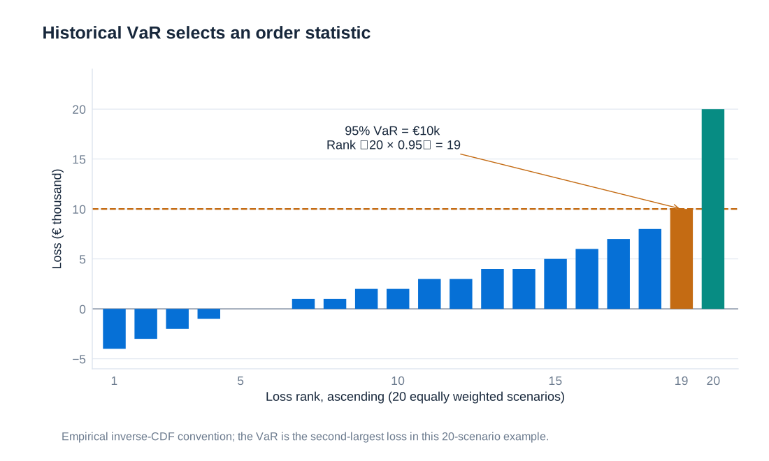
Historical simulation does not require a specific parametric density, but it still assumes that the chosen history is informative about future shocks. It retains only the skewness, tails and dependence present in that sample. A short window may omit a crisis; a long window may mix obsolete regimes with current conditions. Structural breaks, new instruments and missing price histories can make the sample unreliable. Full revaluation captures nonlinear option responses; a historical simulation using only delta approximations does not automatically capture gamma merely because its scenarios are historical.
Variance–covariance and delta–gamma approaches
Let be a vector of risk-factor changes, with mean vector and covariance matrix . Let be the monetary sensitivity of portfolio profit to factor , so the first-order approximation is . For percentage-return factors, is a currency exposure per unit decimal return; for rate changes, it must match the rate unit. The variance is:
The diagonal elements of are factor variances; off-diagonal elements are covariances. If the factor vector is jointly multivariate normal, a linear combination is normal and the delta-normal VaR is . Marginal normality of each factor alone is insufficient: their joint dependence must be specified. Correlations are a major source of diversification, and changes in them can materially alter the result even if each volatility stays fixed.
For an illustrative two-position portfolio, let each position have one-day profit standard deviation EUR 100,000 and correlation 0.5. Portfolio standard deviation is . With zero expected profit, 99% normal VaR is approximately EUR 402,935. If correlation becomes 1, standard deviation rises to EUR 200,000 and VaR to EUR 465,270. The diversification benefit is conditional on dependence, not a permanent property of holding two positions.
A delta–gamma approximation adds the Hessian matrix of second derivatives: . Even when is jointly normal, this quadratic profit is generally not normal. Its quantile may require simulation or a specialised quadratic-form method. Adding gamma and then mechanically multiplying a standard deviation by 2.3263 does not generally produce an exact 99% quantile.
The delta-normal method is fast, transparent and useful for hedge comparisons because it has a closed-form calculation without Monte Carlo sampling error. Its limitations are the linear valuation approximation and the chosen distribution, covariance estimates and factor mapping. Eliminating simulation error does not eliminate parameter uncertainty or model risk. For large option books, fast approximations should be compared with full revaluation under meaningful stresses.
Monte Carlo simulation and the source of simulation error
Monte Carlo simulation specifies a joint probability model, generates many scenarios, values the current portfolio in each and reads the desired quantile from the simulated losses. A run of 10,000 scenarios is a possible starting point, not an assurance of accurate extreme-tail estimates. The method may use normal, heavy-tailed, skewed, jump or other models where justified; normality is not inherent in simulation.
For a multivariate normal example, draw independent standard normal variables , choose a matrix satisfying , and set . A Cholesky factor can be used when the covariance matrix is suitable. Independent draws for the components of do not imply independent simulated factors: the matrix transformation introduces the chosen dependence. Each scenario then feeds a consistent pricing model, producing a monetary portfolio loss.
Full pricing can represent nonlinear options, while path-dependent instruments require simulated paths rather than only terminal shocks. A scenario distribution and valuation model must also be kept conceptually separate: market-risk probabilities usually describe real-world future changes, while option values within each scenario may be calculated using risk-neutral pricing assumptions. Confusing the two probability roles can distort the loss distribution.
Simulation error remains because the scenario sample is finite. At 99% confidence, 10,000 draws leave only about 100 observations beyond the estimated threshold. Results can be checked across independent runs or with appropriate uncertainty estimates, and more draws may improve precision. A fixed random seed supports reproducibility but does not establish accuracy. Parameter misspecification, missing factors and wrong pricing persist even with millions of scenarios. The computational flexibility must therefore be matched by calibration, validation and clear documentation.
Volatility clustering, weighting, EWMA and GARCH
Financial return distributions often have heavier tails and asymmetry relative to a fitted normal distribution. Large absolute returns also tend to cluster: turbulent periods follow turbulent periods, and quiet periods follow quiet periods. A single unconditional standard deviation can consequently describe neither regime well. Empirical histograms and return histories are evidence about these features, not a proof that one alternative model will always forecast them correctly.
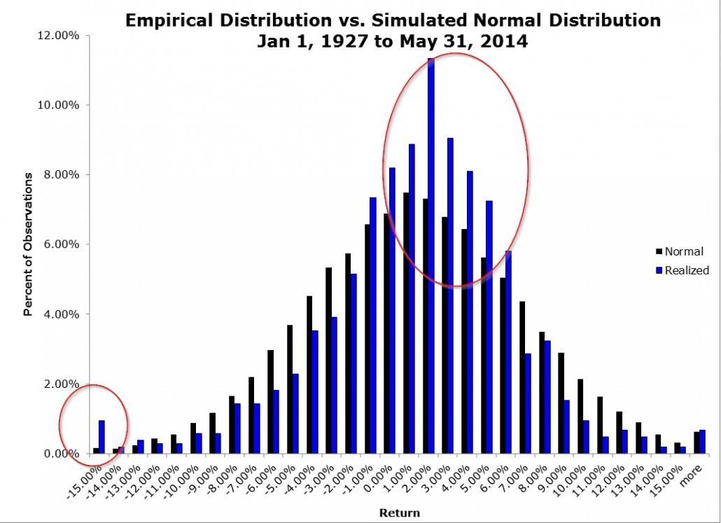
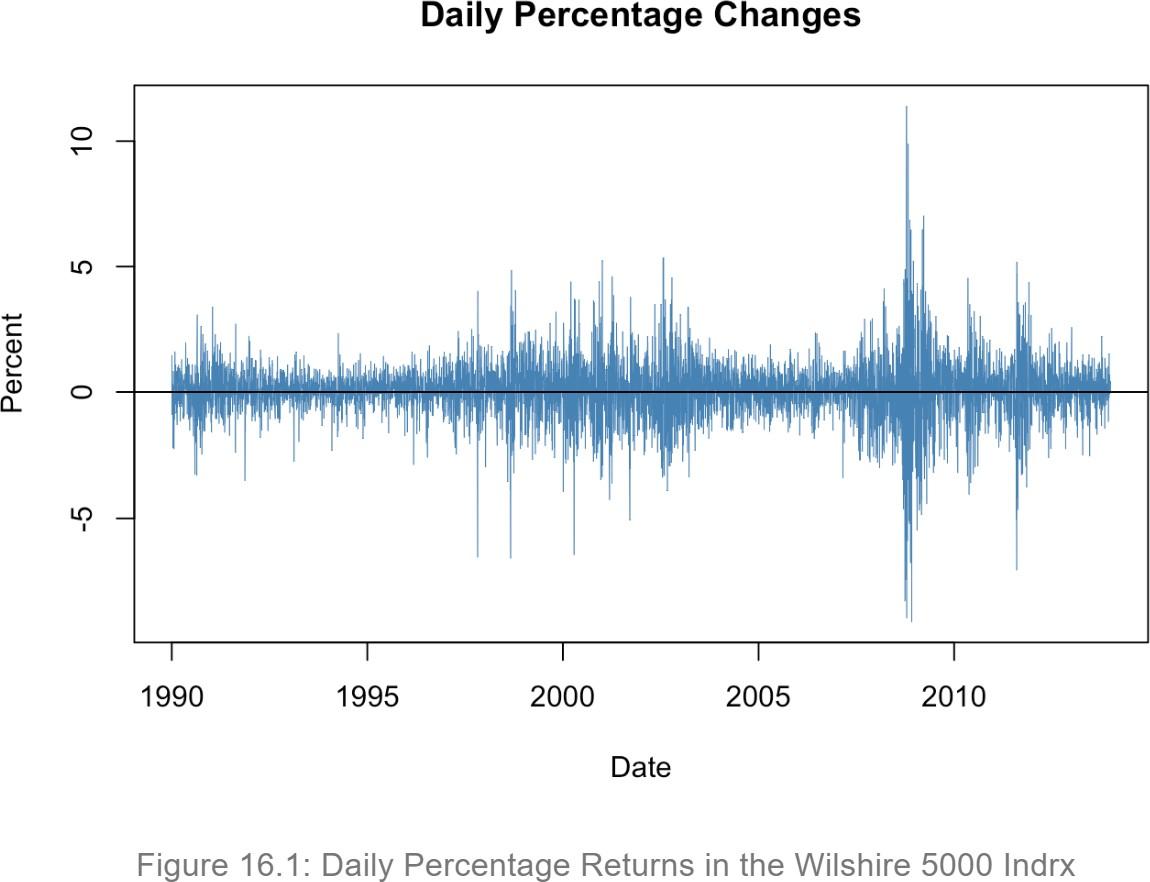
Historical weighting gives recent observations greater influence. For an exponentially weighted moving average, or EWMA, a zero-mean innovation updates the variance forecast as:
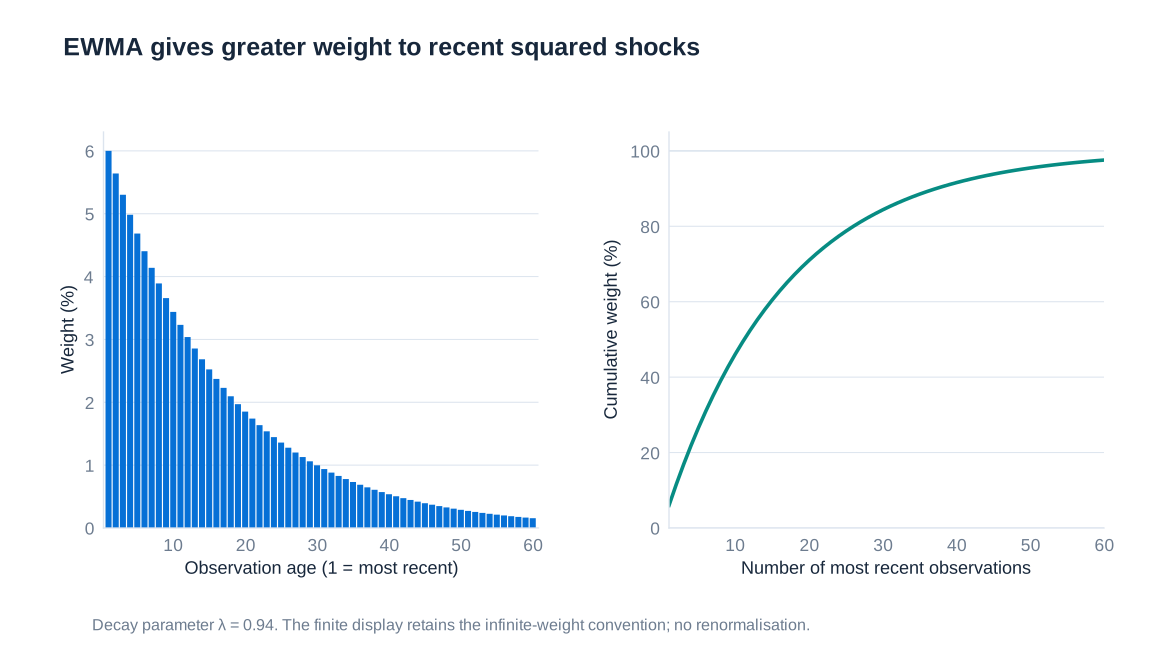
A smaller responds faster to new observations and forgets earlier shocks more quickly. In an illustrative daily model with , current volatility 1% and latest innovation 3%, the next variance is . The next volatility is therefore about 1.2166%, not the weighted average of 1% and 3%. Variances, rather than standard deviations, are being updated.
Ignoring the finite-sample initialisation term, an observation periods back receives weight . At 0.94, the most recent twenty observations carry about 70.99% of the infinite-history weight, and the most recent fifty about 95.47%. A finite window requires consistent normalisation or retention of the initial-variance contribution. Weighted historical quantiles use cumulative scenario weights rather than the unweighted rank formula.
A GARCH(1,1) model adds a constant and separates the shock and persistence coefficients:
For a finite constant unconditional variance in the usual model, , giving . With illustrative values , , , current variance 0.0001 and innovation 0.03, the next variance is 0.000164 and volatility about 1.2806%. The long-run variance is 0.0001. EWMA corresponds to the special zero-intercept recursion with shock and persistence coefficients summing to one, so it does not have this finite mean-reverting variance formula.
These methods forecast conditional volatility; they do not automatically remove skewness, jumps or fat tails from standardised innovations. Filtered historical simulation rescales historical standardised shocks by current volatility forecasts, with dependence and multivariate rescaling treated consistently. A model that adapts rapidly to volatility can still underestimate a new regime, and its forecasts should be compared with stresses that are not mechanically limited to recent experience.
Tail severity, Expected Shortfall and diversification
VaR can remain nearly unchanged when a loss beyond the chosen quantile becomes much larger. Selling a far out-of-the-money put illustrates the problem: most days may show small premium income or modest valuation changes, while a collapse of the underlying creates a severe loss. The premium is compensation for an exposure, not evidence that the exposure has disappeared. A sample without a crash can report very low VaR for a strategy whose economic tail is substantial.
For an integrable loss distribution, Expected Shortfall averages quantiles in the worst fraction:
With a continuous distribution this equals under the usual tail conditions. For a discrete distribution with probability mass at the VaR threshold, the simple conditional expectation can be wrong: the quantile-average definition includes the appropriate fraction of the threshold mass. In the twenty-scenario illustration, 95% VaR is 10 thousand and ES is 20 thousand because the worst 5% is one observation.
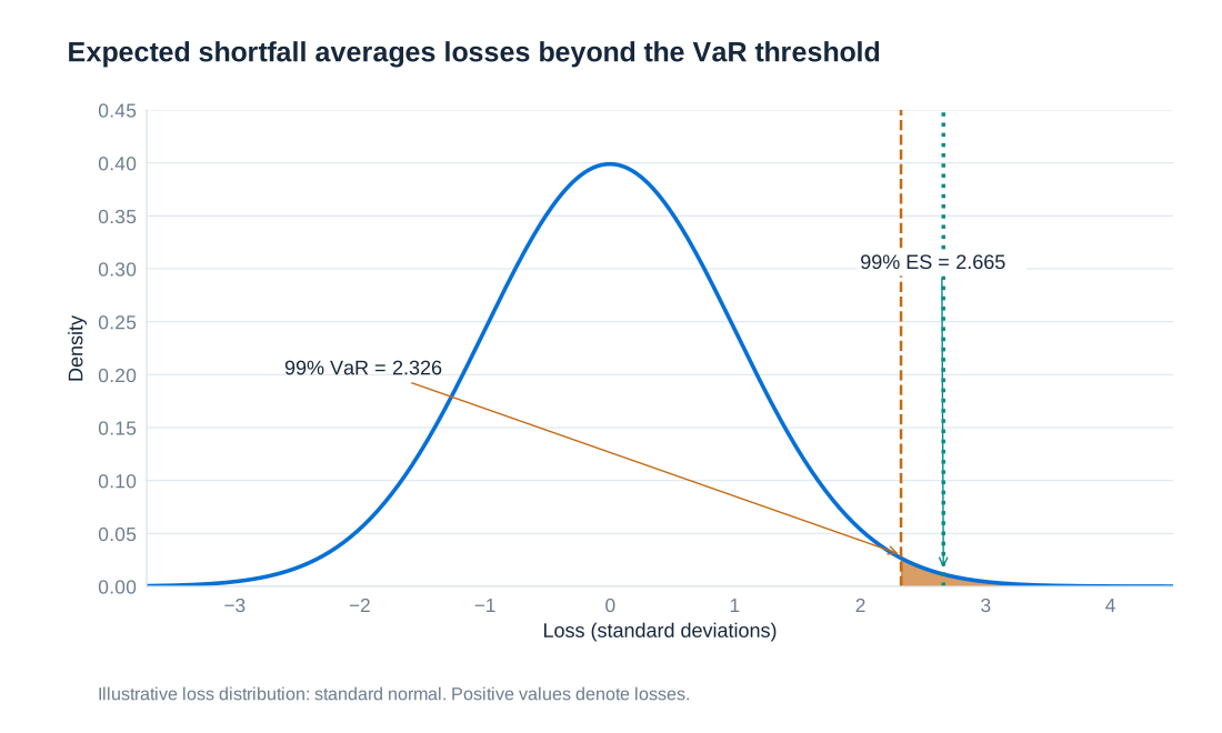
For normal loss , , where is the standard normal density. With mean zero and unit standard deviation, 99% VaR is about 2.3263 and ES about 2.6652. ES describes severity beyond the quantile; it is still model-dependent and is not a worst-case bound.
VaR is not subadditive for every loss distribution. Consider two independent positions, each losing 100 with probability 4% and zero otherwise. Each has 95% VaR zero because a zero loss occurs with probability 96%. Together, the probability of no loss is , so the combined 95% VaR is 100, exceeding the sum of the standalone VaRs. This counterexample does not imply that diversification always increases VaR; it shows that VaR does not universally reward it. ES is subadditive for integrable losses and, together with monotonicity, positive homogeneity and cash-translation behaviour, is a coherent risk measure.
Quiet samples, carry trades and the Niederhoffer case
A carry trade borrows in a low-interest-rate currency and invests in a higher-interest-rate currency without fully eliminating exchange-rate exposure. An illustrative USD-funded Thai-baht investment earning 12% while funding costs 6% appears to earn a 6-percentage-point spread if the exchange rate is unchanged. The interest differential is not a risk-free arbitrage. If the baht value in dollars falls 20% over the year, one borrowed dollar produces dollars of investment proceeds but requires 1.06 dollars of repayment, a loss of 0.164 dollars before other costs.
Thailand allowed the baht to float on 2 July 1997, after pressure on its exchange-rate arrangement. This date must be distinguished from the sharp US equity-market fall on 27 October 1997 and from the timing of individual fund losses. A previously stable exchange rate can produce a low historical volatility estimate until the regime changes. A narrow calibration window may therefore mistake the absence of a past break for the absence of future currency risk.
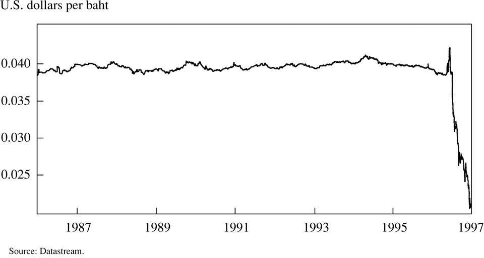
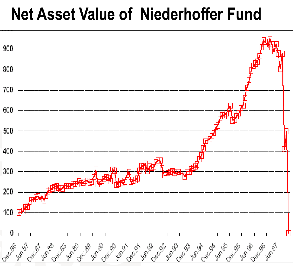
Victor Niederhoffer’s 1997 fund collapse provides a related warning about strategies with strong historical returns and severe exposure to exceptional market moves. It should not be reduced to a single elementary currency carry calculation: option exposures, leverage, market movements and funding pressures can interact. A high historical Sharpe ratio, which compares excess return with volatility, may be uninformative about rare losses when the observation window contains mainly premium income or a stable regime.
The general problem is model risk at several levels: volatility and correlation estimates are uncertain; the assumed distribution may miss jumps or tail dependence; and valuation may be inaccurate precisely in stressed markets. Sensitivity to alternative windows, distributions and correlations should be visible. Stress testing asks how a plausible severe scenario would affect the portfolio even if the fitted probability model assigns it little weight. Reverse stress testing starts from an unacceptable loss and asks which combinations of events could produce it.
Historical source: IMF, Thailand stand-by credit release (1997).
Backtesting, implementation controls and the London Whale
Backtesting compares a forecast made using information available at the time with the subsequent outcome. For a 99% daily VaR, the exception indicator is . A well-calibrated model should have an appropriate exception rate, but frequency alone is insufficient: exceptions clustered during crises reveal conditional misspecification even if the long-run count looks acceptable. Actual trading profit and hypothetical profit on an unchanged portfolio answer different validation questions because new trades, fees and intraday decisions can affect realised results.
The London Whale episode at JPMorgan in 2012 illustrates why implementation and governance matter alongside the statistical formula. The US Senate investigation reported that a new CIO model reduced measured VaR by approximately 50% on introduction, while the positions had not thereby become safer. It identified manual operations, calculation and implementation errors and weaknesses in model review. The broader case also involved risk-limit responses and valuation controls. Attributing the entire loss to a single typographical error would obscure these interacting failures.
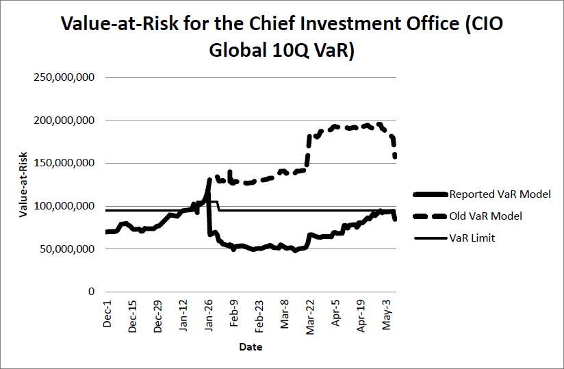
Independent validation should examine whether mathematical specifications are implemented faithfully, compare old and new models on the same positions, reconcile input data and review abrupt risk-number reductions. A lower estimate is not itself evidence of an improved model. Material model changes need a documented economic explanation, independent challenge and clear treatment of existing limits. Sensitivity analysis, stress results and position concentrations should remain available even when a preferred VaR model produces a reassuring number.
Investigation: US Senate, JPMorgan Chase Whale Trades report (2013).
Time horizons, liquidity and the evolution of market-risk regulation
If daily profit increments are independent and identically distributed with mean and variance , their sum over days has mean and variance . With normal increments and stable exposures:
When the mean is negligible, ten-day normal VaR is approximately times one-day VaR, not ten times. Independence and identical distributions alone establish variance scaling when variance exists; they do not make every distribution’s quantile scale exactly with the square root of time. Serial dependence, changing volatility, nonlinear valuation, jumps, rebalancing and liquidation costs can invalidate the shortcut. A position that cannot be sold quickly also remains exposed beyond a nominal one-day reporting horizon.
J.P. Morgan publicly launched RiskMetrics in 1994. The Basel Committee’s 1996 Market Risk Amendment introduced a framework permitting standardised market-risk capital calculations and approved internal models. Post-crisis reforms included the 2009 Basel 2.5 changes and stressed VaR. The Fundamental Review of the Trading Book, or FRTB, subsequently centred the internal-model framework on stressed ES and liquidity risk. The ECB’s Targeted Review of Internal Models, or TRIM, is a separate supervisory review initiative; interest-rate risk in the banking book also has its own supervisory framework rather than simply being absorbed into trading-book VaR.
The Basel market-risk standard uses 97.5% one-tailed ES and a ten-day base horizon, with specified liquidity-horizon categories extending to 120 days. The following mapping summarises the risk-factor categories in that framework; it describes the standard, not a claim that every jurisdiction applies every provision on an identical implementation date. IG denotes investment grade and HY high yield.
| Risk-factor category | Horizon |
|---|---|
| Interest rates: specified currencies and a bank’s domestic currency | 10 |
| Interest rates: other currencies | 20 |
| Interest-rate volatility and other interest-rate factors | 60 |
| Sovereign credit spreads: IG | 20 |
| Sovereign credit spreads: HY | 40 |
| Corporate credit spreads: IG | 40 |
| Corporate credit spreads: HY | 60 |
| Credit-spread volatility and other credit-spread factors | 120 |
| Large-cap equity prices | 10 |
| Small-cap equity prices and large-cap equity volatility | 20 |
| Small-cap equity volatility and other equity factors | 60 |
| FX rates: specified currency pairs | 10 |
| FX rates: other currency pairs | 20 |
| FX volatility and other FX factors | 40 |
| Energy and carbon-emissions prices | 20 |
| Precious and non-ferrous metal prices | 20 |
| Other commodity prices | 60 |
| Energy, carbon-emissions, precious and non-ferrous metal volatility | 60 |
| Other commodity volatility and other commodity factors | 120 |
The specified interest-rate currencies include EUR, USD, GBP, AUD, JPY, SEK and CAD, together with the bank’s domestic currency. Exact FX-pair eligibility and supervisory adjustments require the framework’s definitions. Liquidity-adjusted ES aggregates exposures assigned to different horizons; it is not obtained by multiplying the entire portfolio by its longest horizon. Modelling the availability and quality of market observations is also necessary, because stale or sparse prices can make apparently precise factors unsuitable for the normal modelling process.
Regulatory references: Basel Framework MAR33; Basel Committee, market-risk capital requirements (2019).
Model heterogeneity and the limits of a single number
Even when institutions value the same positions, different data windows, dependence assumptions, pricing approximations and implementation choices can generate materially different capital estimates. The Basel Committee’s 2013 regulatory consistency assessment reported the following results for a common diversified test portfolio. The figures are historical model-comparison evidence, not current capital requirements for an investor’s portfolio.
| Statistic across models | Reported value |
|---|---|
| Minimum | EUR 13,414,208 |
| Maximum | EUR 34,165,014 |
| Median | EUR 17,781,481 |
| Mean | EUR 20,521,469 |
| Standard deviation | EUR 6,344,392 |
| Standard deviation divided by mean | 31%, rounded |
The maximum is more than twice the minimum. This dispersion is a reason to investigate model choices, not proof that the smallest or largest estimate is automatically correct. Regulatory capital incentives can create pressure to favour low measured risk, making independent governance especially important. Harmonised definitions, validation, benchmarking and credible standardised alternatives help constrain unjustified differences.
A useful risk report therefore places VaR and ES beside stress losses, sensitivities, liquidity assumptions, concentrations and model limitations. VaR supplies a common threshold language; ES adds tail severity; neither removes the need to understand the positions. The quality of market data, valuation, implementation and escalation determines whether the resulting numbers support decisions or merely give false precision.
Historical comparison: Basel Committee, analysis of market-risk weighted assets (2013).