
1. Financial risk, governance and stock-market exposure
Financial risk management connects uncertain outcomes with decisions about investment, financing and the survival of an institution. Its purpose is to understand which risks a business takes, whether their potential rewards justify them, and whether losses can be absorbed when conditions deteriorate. Eliminating every risk would also eliminate many productive activities. The practical objective is to choose exposures deliberately, measure them appropriately and maintain the financial and organisational capacity to withstand adverse outcomes.
Recognising the different sources of risk
Market risk arises when movements in prices or rates change the value of a position. Equity prices, interest rates, exchange rates and commodity prices are distinct market factors, but a single transaction can expose a business to several of them. A dollar-denominated bond held by a euro-based investor has interest-rate exposure and currency exposure; if the issuer can default, it also has credit exposure. Describing it simply as a bond does not identify the risks that determine its value.
Credit risk concerns failure to receive contractual payments and deterioration in a counterparty's ability to pay. Default probability matters, but so do the amount owed at default, the recovery available, concentration in particular borrowers or industries, and country conditions that can impede repayment. Liquidating collateral may take time and yield less than its recorded value. A large number of loans can still constitute a concentrated portfolio when borrowers depend on the same economic conditions.
Liquidity risk has two connected dimensions. Funding liquidity is the ability to meet payments and refinance obligations when due. Market liquidity is the ability to sell or hedge an asset without an excessive price concession. A solvent-looking institution can fail if it cannot raise cash quickly enough. Conversely, forced sales made to obtain cash can crystallise losses and weaken capital. The distinction between a loss of value and a shortage of immediately available money is therefore fundamental.
Operational risk includes failures of processes, people, technology and internal controls, as well as external events. Legal and compliance failures can produce fines, compensation obligations and restrictions on business. Strategic or business risk concerns the viability of the business model, competitive position and choices about products and markets. Reputational damage can amplify any of these risks by undermining customer, investor or counterparty confidence. The categories organise analysis; they do not imply that actual losses respect organisational boundaries.
Systemic risk concerns disruption of the financial system rather than only the failure of one institution. Common exposures, interconnected claims and simultaneous attempts to sell assets can transmit problems across firms. Model risk arises when decisions rely on an inappropriate model, unreliable inputs or assumptions that no longer describe the environment. Incentive risk arises when a decision-maker benefits from taking risks whose costs fall elsewhere. A distressed firm's shareholders may prefer a gamble that offers a chance of recovery while transferring much of the downside to creditors, deposit insurers or taxpayers. This is the logic of gambling for resurrection.
The risk-management cycle and the choice of response
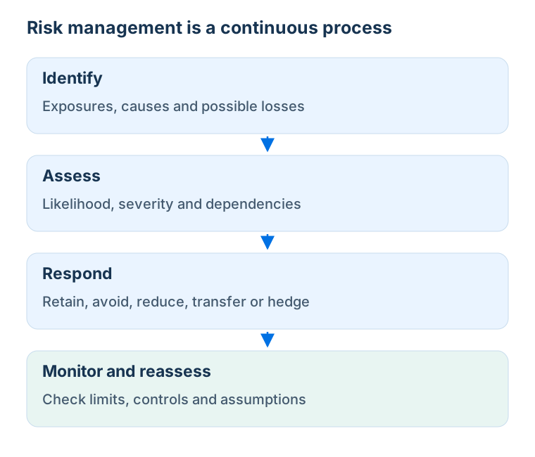
A useful risk-management process begins with identification: what could go wrong, through which mechanism and for whom? Internal incidents, external failures and structured self-assessment help reveal exposures that are not apparent from a balance sheet. Assessment then connects causes to financial consequences, identifies the amount exposed, and estimates the frequency and severity of losses where quantification is credible. A rare loss capable of threatening survival deserves attention even if its expected annual cost looks small.
The institution next chooses controls and limits consistent with its risk appetite. An exposure limit constrains the amount at risk; a concentration limit prevents dependence on a single source of repayment; a loss or capital limit constrains the consequences of adverse scenarios. Finally, monitoring tests whether the controls work, whether limits are respected and whether the original assumptions remain valid. New information should feed back into identification and assessment. A policy that is written once and never challenged is not a complete risk-management system.
Risk can be retained when its size is acceptable and the institution can absorb it. Retention should be a conscious decision rather than the accidental result of failing to measure an exposure. Avoidance removes the activity generating the risk, for example by leaving a market or closing a business line. Reduction changes the probability or severity of a loss: better information systems reduce processing failures, while collateral may reduce the loss associated with a borrower's default.
Risk transfer reallocates consequences through insurance, contractual indemnities, outsourcing or other agreements. Outsourcing a process does not remove responsibility for overseeing it, and insurance creates its own exclusions, limits and counterparty dependence. Hedging uses offsetting financial positions, such as futures, options or credit derivatives. It can reduce the sensitivity of a portfolio to a specified risk factor while introducing basis risk, collateral needs or counterparty exposure. The relevant question is how the combined position behaves, not whether the hedge itself ever loses money.
A risk manager need not personally program every calculation, but must understand what the model measures, specify the analysis required and interpret its limitations. Specialist software and AI tools can assist with calculations and explanations, yet their output still needs checking against definitions, units, known examples and reliable sources. A plausible-looking formula or chart can be wrong. Independent reproduction of a material result is particularly valuable when the conclusion affects capital, limits or investment decisions.
Governance, independent control and the three lines
The three-lines framework assigns different responsibilities to the people who take risk, those who challenge it and those who provide independent assurance. The first line consists of operating management and the business units that originate transactions. They own the risks of their activities and must maintain effective day-to-day controls. The second line includes risk management and compliance functions that establish frameworks, monitor exposures and challenge decisions. These functions require sufficient authority, expertise and access to information to disagree with revenue-generating teams.
Internal audit forms the third line. It assesses whether governance, risk management and controls are designed and operating effectively, and reports independently to the governing body or its audit committee. The board oversees strategy and risk appetite; senior management implements them. External audit and supervision supply additional scrutiny, but neither replaces the institution's own lines of responsibility. A diagram with three boxes is ineffective if staff cannot escalate concerns or if managers can alter the information presented to the board.
Independence matters especially when performance is rewarded through short-term profits. A trader can earn an attractive return by selling protection against an infrequent catastrophe: profits appear stable until the adverse event occurs. If the trader also determines the reported risk and can change loss scenarios, both the apparent return and the apparent risk may be misleading. Controls should therefore protect valuation, model validation and communication of risk information from manipulation by the people whose performance is being assessed.
Effective oversight also requires understanding the economic purpose of a transaction. A derivative loss can be consistent with a successful hedge if the underlying exposure gains value. Equally, a profitable derivative position can conceal a dangerous increase in unhedged risk. Boards need reports that combine exposures, hedges, funding requirements and stress outcomes, with clear explanations of assumptions and exceptions.
Legal reference: German Banking Act, section 54a.
Catastrophe bonds and the distinction between an event and a valuation loss
Catastrophe bonds illustrate why risk knowledge matters beyond trading desks and banks. These securities transfer specified disaster losses to investors. Their terms define triggers, such as a particular insured loss, an industry loss measure or a physical characteristic of a hurricane or earthquake. Investors receive compensation for accepting the possibility that interest or principal will be reduced when the contractual trigger is met. The exact trigger and the assets securing the obligation must be understood before interpreting the coupon as an investment return.
The absence of a trigger does not guarantee a stable market price. Investors may revise the estimated probability of a disaster, demand a higher risk premium, reassess the quality of catastrophe models or need to sell into an illiquid market. A bond can consequently lose market value without yet suffering a contractual principal write-down. An institution investing money needed for predictable future commitments must consider this valuation and liquidity risk as well as the trigger probability.

The same distinction applies to apparently safe banking assets. A government bond may retain a high probability of repayment at maturity while losing substantial market value when interest rates rise. Whether the holder can wait until maturity depends on its liabilities and available liquidity. A promise of eventual repayment does not solve an immediate funding problem.
A banking failure need not appear as an ordinary corporate bankruptcy. A bank may be resolved, sold, merged or supported through an institutional protection arrangement. A June 2025 report on Raiffeisenbank im Hochtaunus described an expected EUR 1.2 billion support burden for the cooperative banking protection scheme and identified it as a further case within that sector. The relevant lesson is that intervention can prevent a disorderly closure while still revealing serious losses and weaknesses in the failed institution's risk management.

Silicon Valley Bank: interest-rate risk, liquidity and incentives
Silicon Valley Bank's March 2023 failure demonstrates how several risks reinforce one another. Rapid deposit growth financed a large portfolio of longer-duration securities. When interest rates rose, the market value of those securities fell. The bank also relied heavily on concentrated, uninsured deposits whose owners could withdraw funds quickly. A portfolio that appears manageable under an assumption of stable funding becomes much more vulnerable when funding leaves and assets must be monetised.
The Federal Reserve's 2023 review found weaknesses in governance, liquidity planning and interest-rate-risk management. It described management's focus on short-run earnings, breaches of longer-term interest-rate-risk limits and the removal during 2022 of hedges that would have helped protect against rising rates. Realising a gain on a hedge does not create protection against the next adverse movement: after the position is closed, the exposure it offset remains unless another adjustment replaces it.
Compensation was part of this governance problem. Supervisors found that incentive decisions relied heavily on financial performance and gave insufficient weight to risk-management deficiencies. This supports a lesson about incentives and accountability. It does not establish the stronger claim that particular managers removed particular swaps solely to obtain a specified bonus, or that bonuses alone caused the failure. A careful explanation distinguishes documented weaknesses from an inferred personal motive.
The immediate crisis involved a loss of depositor confidence, a securities sale that crystallised losses and exceptionally rapid withdrawals. The bank was closed on 10 March 2023. The broader lesson is that interest-rate risk, funding concentration, unrealised losses and inadequate contingency arrangements cannot be analysed in isolation. Accounting classifications may affect when losses appear in reported earnings, but they do not remove the economic loss or the cash needed to meet withdrawals.
Primary sources: Federal Reserve review of SVB, risk management (2023); Federal Reserve review of incentive compensation (2023).
Investment mandates, misconduct and supervisory intervention
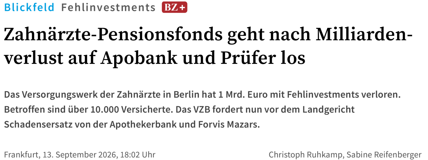
The Berlin dentists' pension institution, VZB, provides a different governance setting. Retirement promises require investment decisions consistent with liquidity needs, diversification and the institution's mandate. Contemporary reporting described very large losses and disputed exposure to risky, illiquid investments. Claims against former managers, advisers, auditors or supervisory bodies concern different duties and require separate evidence. A risk report produced by an outside provider does not, by itself, establish that the governing body discharged its own responsibilities.
The Berlin Labour Court confirmed in July 2026 that VZB sought approximately EUR 50 million in damages from its former director and that procedural questions remained before the court. That is a confirmed claim, not a final finding of liability. Reported portfolio percentages, total loss estimates and the number of people under investigation should not be treated as settled judicial facts. The study lesson is the danger of allowing an investment mandate, actual portfolio risk and independent oversight to diverge, together with the importance of distinguishing allegations, valuations and adjudicated responsibility.
The Allianz Global Investors US Structured Alpha case involved a documented fraud in which investors were misled about downside protection and risk. Altered risk information and misrepresented hedging practices prevented investors from understanding the exposures they accepted. Following a guilty plea, the July 2023 sentence included more than USD 463 million in forfeiture, USD 3.23 billion in restitution and USD 2.33 billion in fines. Describing the entire resolution as a single fine for breaching a three-lines diagram is inaccurate: the underlying misconduct and the categories of financial sanction matter.
N26 illustrates how compliance weaknesses can restrict business growth. BaFin imposed measures relating to anti-money-laundering controls, appointed special monitoring and restricted customer acquisition. The historical growth restriction began in 2021 and was lifted effective June 2024, according to N26's announcement. Separate fines of EUR 4.25 million in 2021 and EUR 9.2 million announced in 2024 concerned delayed suspicious-activity reporting. The economic cost of deficient controls includes remediation expenditure and lost business opportunities, as well as the fine itself.
German banking law also makes specified failures of risk governance potentially relevant to criminal responsibility. Section 54a KWG provides for imprisonment of up to five years or a fine in the circumstances it defines. The offence requires more than an investment loss: it connects specified management duties, a binding supervisory remediation order and an ensuing threat to the institution's continued existence. Negligently causing the specified danger is treated separately. Risk management is therefore both an economic discipline and a set of responsibilities whose legal consequences depend on the facts and applicable provisions.
Case documentation: US Department of Justice, Structured Alpha sentencing (2023); Berlin Labour Court, pension-fund proceedings (2026); BaFin, N26 restrictions (2021); N26, fine disclosure (2024); N26, removal of the growth restriction (2024).
Recurring lessons from historical failures
Financial history contains repeated examples of familiar exposures interacting with leverage, liquidity and weak controls. The US savings-and-loan crisis exposed the vulnerability of institutions funding long-term assets with liabilities whose cost could rise much faster. Metallgesellschaft's 1993 oil-related difficulties showed that a hedge can generate severe intermediate cash requirements when the maturity and settlement pattern of derivatives differ from the commercial contracts being hedged. The lesson is not that all hedging is dangerous, but that funding the hedge is part of its design.
Long-Term Capital Management in 1998 combined leveraged positions with assumptions about market relationships and liquidity that became unreliable under stress. The episodes involving Nick Leeson at Barings in 1995 and Jérôme Kerviel at Société Générale in 2008 illustrate the importance of trade verification, position limits and separation of duties. JPMorgan's 2012 London Whale losses involved complex credit derivatives and weaknesses in oversight and risk reporting. A model's numerical output cannot substitute for a clear understanding of the position it describes.
Lehman Brothers' failure in 2008 intensified an already developing global financial crisis; it did not single-handedly initiate every aspect of that crisis. Exposure to mortgage-related assets, leverage and fragile funding were central concerns. Cum-ex transactions, in contrast, illustrate legal and conduct risk arising from arrangements associated with improper tax refunds. These cases should not be reduced to one interchangeable story about volatility. Their common feature is that a narrow view of reported profit or a single risk metric failed to capture the full consequences of the activity.
Loss distributions, Value at Risk and Expected Shortfall
Let denote the monetary loss over a specified horizon, with positive values representing losses and negative values representing gains. A risk measure summarises some feature of its distribution. Variance measures dispersion around the mean; it treats favourable and adverse deviations symmetrically. Maximum possible loss asks for the worst outcome permitted by the position's payoff. It can be limited for an unleveraged long investment, but unbounded in an idealised model for certain short positions. Neither quantity is interchangeable with a high-confidence loss quantile.
Value at Risk at confidence level is the loss quantile:
A one-day 99% VaR of USD 1 million means that the model assigns approximately 1% probability to a loss above USD 1 million over one day. It is not the maximum loss that can occur. The horizon, confidence level, valuation convention and assumptions about the portfolio must accompany the number. A 95% annual VaR and a 99% daily VaR answer different questions and cannot be compared simply by looking at their monetary amounts.
Expected Shortfall, also called ES or CVaR, measures the average loss in the worst tail. A definition that also handles distributions with discrete probability masses is:
For a continuous loss distribution, this is the expected loss conditional on being beyond the VaR threshold. ES distinguishes portfolios with the same VaR but very different losses in extreme scenarios. It also requires information about a part of the distribution where data are scarce and modelling assumptions are consequential. A precise-looking tail estimate should therefore be read together with stress tests and model limitations.
A stress test asks how a portfolio or institution performs under a specified adverse scenario: for example, a recession combined with higher defaults, falling collateral values and stressed funding. It need not assign that scenario a precise probability. A supervisory stress result showing a reduced capital ratio is conditional on the scenario and methodology, not a forecast that the bank will fail with that ratio. Published rankings are meaningful only after the starting position, projected losses and scenario assumptions are understood.
For example, LBBW's published 2025 exercise reported a transitional CET1 ratio of 6.82% at the end of the adverse 2027 scenario, compared with a restated starting ratio of 16.85%. Its fully loaded adverse ratio was 5.54%, using a different regulatory basis. These are scenario outcomes under specified capital rules, not alternative observations of an actual future capital ratio. Mixing transitional and fully loaded figures, or ignoring the restatement of the starting position, produces misleading comparisons.
Maximum drawdown supplies a complementary path-based measure. If is portfolio value and is its previous peak, percentage drawdown is and maximum drawdown is the largest such decline over the observed interval. It depends on the sequence of values, unlike a single terminal-return quantile. Historical maximum drawdown is the worst peak-to-trough decline in that history, not a bound on the losses that could occur in the future.
Expected loss, unexpected loss and economic capital
For a simple credit exposure, expected loss is commonly represented as:
PD is the probability of default over the chosen horizon, LGD is the fraction of exposure lost conditional on default, and EAD is the monetary exposure at default. The expression is exact when LGD and EAD are fixed conditional inputs. With stochastic exposures and recoveries, dependence must be handled consistently rather than multiplying unrelated unconditional averages. At portfolio level, expected loss is .
Unexpected loss is used in more than one way. Here, denotes the standard deviation of portfolio credit losses. It measures dispersion around expected loss. Economic capital is a separate tail-based quantity: the buffer intended to absorb losses above the expected amount up to a selected confidence level:
At 99.95% confidence, the model assigns 0.05% probability to losses beyond the selected threshold. That percentage is not the standard deviation and should not be called an amount of unexpected loss without specifying the convention. Economic capital is also a modelling and management concept; it need not equal regulatory capital.
Expected credit losses should be incorporated into lending prices, provisioning and the assessment of profitability. Capital is then intended to absorb adverse deviations beyond the loss already expected and allowed for. This is the economic logic behind saying that lending customers pay for expected loss through risk-adjusted interest rates. It is not a guarantee that expected losses have already been collected in cash or fully provisioned. Underpricing, unexpected changes in default risk and accounting timing can leave a real shortfall.
Risk-weighted assets and the role of regulatory capital
Risk-weighted assets, or RWA, translate different regulated exposures into a common denominator for capital ratios. Credit, market and operational risks contribute through their respective regulatory calculations; off-balance-sheet commitments and derivatives cannot simply be omitted because they are not ordinary loans on the balance sheet. The Common Equity Tier 1 ratio is:
CET1 is a defined regulatory category of high-quality capital after relevant adjustments, not every item described as equity in the accounts. Minimum ratios, buffers and additional requirements determine how the resulting ratio is assessed. RWA is not a forecast of monetary losses and is not identical to total assets. A lower measured RWA can reflect changes in asset composition or regulatory treatment without a proportional reduction in every economic risk.
For credit risk, a standardised approach applies prescribed treatments that may depend on exposure type and eligible external ratings. Internal-ratings-based approaches use permitted bank estimates within a supervisory framework and formula. The following historical rating illustration shows the logic of assigning different weights; it is not a current capital-calculation schedule. The precise rating boundaries, exposure definitions, national implementation and applicable version must be checked before using regulatory weights in practice.
| Exposure category | Highest rating bucket | A range | BBB range | BB/B bucket | Lowest rated bucket | Unrated |
|---|---|---|---|---|---|---|
| Sovereign | 0% | 20% | 50% | 100% | 150% | 100% |
| Bank, historical option 1 | 20% | 50% | 100% | 100% | 150% | 100% |
| Bank, historical option 2 | 20% | 50% | 50% | 100% | 150% | 50% |
| Bank, historical short-term treatment | 20% | 20% | 20% | 50% | 150% | 20% |
| Corporate | 20% | 50% | 100% | 100% | 150% | 100% |
The same historical illustration assigned 35% to the stated residential category, 100% to the commercial category and 75% to other qualifying retail exposures. These figures illustrate the use of exposure classes rather than a universal principle that every residential asset is always weighted at 35%. The heading “unrated” does not mean that all retail exposures fall into a single unrestricted treatment.
A legacy corporate IRB expression makes the relationship between expected loss and capital more explicit. Writing for the standard-normal cumulative distribution and for its inverse, a historical specification is:
Here is a capital requirement per unit of exposure, is the prescribed asset-correlation parameter, is effective maturity in years and is the prescribed maturity-adjustment function. PD and LGD retain their credit-risk meanings. The bracket measures a stressed conditional loss less expected loss; the final fraction adjusts maturity. The corresponding risk-weight conversion is , so in this representation. The 12.5 factor is the reciprocal of 8%. The historical factor 1.06 was removed in the finalised Basel III framework; carrying it mechanically into a current calculation would be incorrect. This introduction explains the structure, while detailed credit-risk modelling requires the applicable parameters and rules.
Regulatory and historical references: Basel III reform summary; LBBW, 2025 stress-test results.
Risk, uncertainty and the shape of distributions
Risk is often used for situations in which probabilities can be estimated with some credibility; uncertainty describes situations in which the relevant mechanisms or probabilities are not reliably known. In the tradition associated with Frank Knight, the distinction matters because adding decimal places to a model does not resolve ignorance about the process generating losses. Familiar credit defaults may be represented by a statistical model. A new geopolitical disruption may require scenarios with uncertain probabilities. An unrecognised failure mechanism calls for resilience and contingency capacity as well as measurement.
The mean is the expected value, . Variance is the second central moment, , and standard deviation is its square root. In financial applications, volatility usually means the standard deviation of returns over a specified horizon or its annualised counterpart. It is essential to state the return definition, frequency and estimation period: daily simple-return volatility is not automatically interchangeable with annual log-return volatility.
Skewness and kurtosis describe features that variance alone misses:
Negative skewness indicates a longer or more influential left tail, while positive skewness indicates the opposite direction. When low returns represent losses, negative skewness warns that adverse outcomes may be more severe than a symmetric approximation suggests. However, skewness alone does not mathematically determine every VaR quantile: the complete distributions and the confidence level matter.
A normal distribution has kurtosis 3, or excess kurtosis zero when 3 is subtracted. Kurtosis above 3 signals a larger standardised fourth moment and often accompanies more extreme observations than a normal model predicts. It is a useful warning about tail-sensitive modelling, but is not a complete description of the tail or a universal ranking of all extreme quantiles. Some heavy-tailed distributions do not even possess a finite fourth moment. Stress analysis is especially valuable when historical data are too sparse to estimate such features reliably.
Portfolio return, covariance and diversification
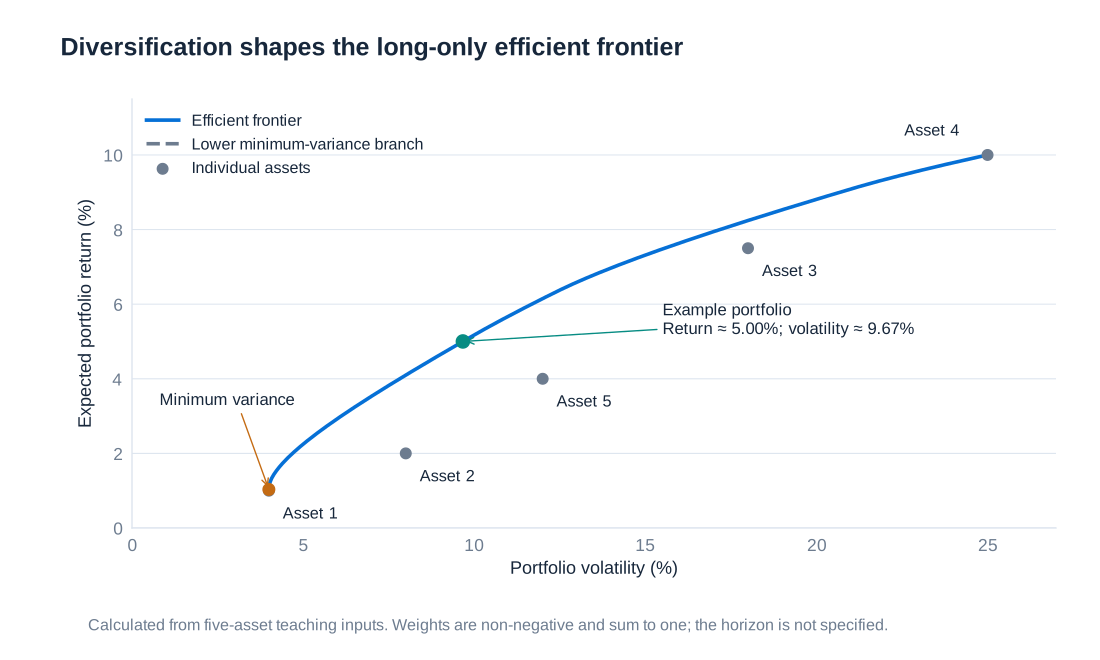
Markowitz portfolio analysis evaluates combinations of expected return and variance. A portfolio lies on the efficient frontier when no feasible alternative offers a higher expected return for the same risk, or a lower risk for the same expected return. Risk aversion does not imply selecting the lowest-volatility asset in isolation. It means choosing an appropriate efficient combination, given the investor's objective and constraints.

Let be the fraction of portfolio value invested in asset , with , and let denote its return. For fixed weights over the measurement period, portfolio return is . If and , then:
The vector contains the weights and the matrix contains covariances. Its diagonal entries are individual variances. Off-diagonal entries satisfy , where is the return correlation. Portfolio risk is therefore not a simple weighted average of individual volatilities. Diversification depends on how assets move together, and a correlation estimated in calm conditions may not describe a stressed market.
| Asset | Expected return | Volatility | Weight |
|---|---|---|---|
| 1 | 1.00% | 4.00% | 3.10% |
| 2 | 2.00% | 8.00% | 21.48% |
| 3 | 7.50% | 18.00% | 23.77% |
| 4 | 10.00% | 25.00% | 11.52% |
| 5 | 4.00% | 12.00% | 40.13% |
The pairwise correlations are , , , , , , , , and . Correlations are symmetric and each asset has correlation 1 with itself. Converting percentage returns to decimals before multiplying gives the following covariance matrix.
| Asset | 1 | 2 | 3 | 4 | 5 |
|---|---|---|---|---|---|
| 1 | 0.001600 | 0.001600 | 0.001440 | 0.003000 | 0.002400 |
| 2 | 0.001600 | 0.006400 | 0.005760 | 0.006000 | 0.000960 |
| 3 | 0.001440 | 0.005760 | 0.032400 | 0.031500 | 0.003240 |
| 4 | 0.003000 | 0.006000 | 0.031500 | 0.062500 | 0.006000 |
| 5 | 0.002400 | 0.000960 | 0.003240 | 0.006000 | 0.014400 |
For example, . Multiplying the expected returns by their weights gives , approximately 5.00%. The quadratic form gives variance 0.0093482194 and standard deviation 0.0966862, approximately 9.7%. These numbers refer to the same horizon as the inputs. A spreadsheet implementation uses a weighted sum for the mean and matrix multiplication for ; the matrix should be symmetric and positive semidefinite. Rounding its entries too aggressively can distort the result.
Normal quantiles and a portfolio VaR calculation
If the vector of asset returns is jointly normal, every fixed linear combination is normal. It is not enough that each asset has an individually normal marginal distribution: the joint dependence structure also matters. Under the joint-normal assumption, . If , then . Approximately 5% of standard-normal observations lie below −1.645 and 5% above 1.645.
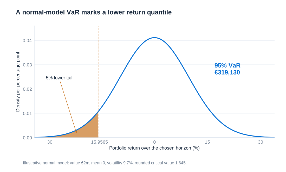
The lower 5% portfolio-return quantile is consequently . For initial value and simple return over the chosen horizon, the corresponding normal loss quantile is:
Loss is measured relative to initial value here. A risk system that measures losses relative to expected value would report a different convention. The formula can also produce a negative loss quantile when expected gains dominate the selected threshold; reporting systems sometimes floor VaR at zero, but that convention should be stated rather than silently changing the mathematics.
| Confidence level | Positive quantile, approximately |
|---|---|
| 50% | 0.000 |
| 84.13% | 1.000 |
| 95% | 1.645 |
| 99% | 2.326 |
| 99.90% | 3.090 |
| 99.99% | 3.719 |
Suppose EUR 2 million is invested and the volatility over the risk horizon is taken as the rounded 9.7%. With expected return assumed zero for this separate VaR illustration, the 95% lower return quantile is . The loss threshold is therefore euros, approximately 15.96% of value. This calculation deliberately uses rounded volatility and a zero mean; it does not simultaneously use the five-asset portfolio's 5% expected return.
The horizon cannot be inferred from the final amount. If 9.7% is annual volatility, the result is an annual-horizon calculation; if it describes another horizon, that horizon applies. Scaling volatility by the square root of time requires assumptions about independent increments and stable variance. Fat tails, changing volatility and nonlinear payoffs can make the normal approximation inadequate even when the arithmetic is correct.
Hedging systematic equity risk with index futures
An equity portfolio's systematic exposure can be measured by beta, , where is the market return. A beta of 0.8 means that a one-percentage-point market movement is associated, in the fitted relationship, with approximately a 0.8-percentage-point portfolio movement. It is a sensitivity, not a guarantee that every realised return follows the index. Firm-specific events and changing relationships remain possible.
A manager holding equities can reduce this exposure by selling appropriate stock-index futures. A short futures position gains when the index falls and loses when it rises. Index hedging can be quicker and less costly than selling every holding or hedging each security separately. The relevant index must resemble the portfolio's market exposure: using a DAX-related contract for German equity exposure and an S&P 500-related contract for US exposure are examples of the matching principle, not universal prescriptions.
For a contract with futures price and multiplier , the notional exposure per contract is . A beta-based number of contracts to sell is:
where is current portfolio value and is the desired remaining beta. A positive denotes contracts sold. For market neutrality, . Contract rounding, differences between the cash index and futures price, and basis changes prevent this formula from being a promise of exact protection.
Consider a USD 30 million portfolio with beta 0.8. Its beta-adjusted market exposure is USD 24 million. Using an illustrative E-mini S&P 500 futures level of 8,000 and a USD 50 multiplier gives USD 400,000 notional per contract, so the hedge sells 60 contracts. A 10% index fall implies an approximate USD 2.4 million systematic portfolio loss and an equal gain on the short futures. The combined systematic exposure is million dollars.
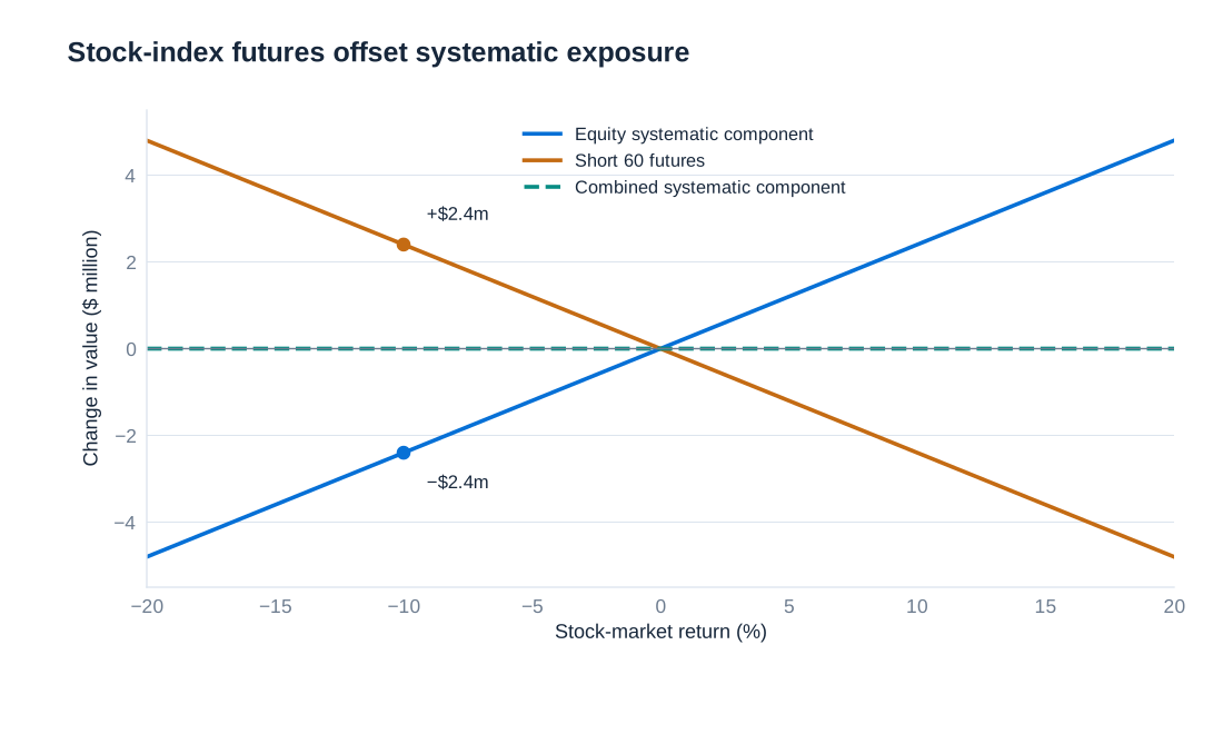
The USD 50 multiplier identifies the particular contract specification used in this example; other contracts have different sizes. A ten-point rise generates a USD 500 gain for the long side and an equal loss for the short side. Cash-settled futures do not require delivery of the underlying shares, and gains and losses are settled through daily variation margin. The familiar quarterly expiry cycle uses March, June, September and December contracts. Holding the hedge requires cash for adverse margin movements even when the combined investment performs as intended.
Market-neutral does not mean risk-free. The portfolio retains idiosyncratic risk, model and beta-estimation risk, basis risk and potentially liquidity risk. Beta can change as positions, prices and business conditions change. A manager must also decide whether to rebalance, roll an expiring contract or tolerate a temporary mismatch. The hedge is successful when it delivers the intended reduction in exposure at an acceptable total cost, not when its derivative leg always reports a profit.
Geometric Brownian motion and positive asset prices
Geometric Brownian motion, or GBM, is a tractable model for a positive asset price. It describes proportional changes rather than adding a normally distributed amount to the price regardless of its level. Its continuous-time specification is:
Here is price or portfolio value at time , is the annualised drift, is annualised volatility, and is a standard Brownian motion. An increment over years satisfies , where . Thus the short-interval approximation is . The random term scales with the square root of time, not time itself.
The exact transition over a finite horizon is:
Equivalently, the log price is normal with mean and variance . The price is lognormal, remains positive and is right-skewed. Finite-horizon simple returns are not exactly normal under this model; normality applies to log returns, while the short-interval proportional-change formula is an approximation. Using the exact exponential update avoids negative simulated prices that a coarse additive approximation could generate.
GBM is useful because its distribution and quantiles can be calculated directly and because it underlies a basic version of option-pricing theory. It remains an assumption. Constant volatility, continuous paths and independent Brownian increments omit volatility clustering, jumps, changing correlations and some features of extreme losses. For real-world risk simulation, drift represents the assumed physical return process. For risk-neutral derivative pricing, the drift is changed consistently with the pricing framework; expected investment return and the risk-free pricing drift should not be interchanged.
Monte Carlo simulation and the interpretation of a risk forecast
Monte Carlo simulation repeatedly draws random inputs and applies the model to generate many possible outcomes. Suppose a portfolio starts at EUR 10,000, with annual drift 9% and volatility 15%, and is projected over five years. A simulation of 10,000 paths can use monthly time steps, , and the exact GBM transition. At each step, every path receives a fresh independent standard-normal draw. The result is a distribution of hypothetical model outcomes, not 10,000 forecasts that the market is expected to follow.
Digital investment services such as Scalable Capital have used distribution-based illustrations to explain possible investment outcomes to clients. The useful feature is the display of uncertainty around a central path rather than a single apparently certain future value. The quality of that communication depends on explaining the return and volatility assumptions and the difference between a model quantile and a promised investment result.
Analytical GBM quantiles provide a direct check on the simulation:
The median corresponds to , whereas the expected value is . These differ because the lognormal distribution is skewed. A middle forecast labelled “50% quantile” is a median, not automatically the mean. The following comparison keeps analytical values separate from the estimates produced by one illustrative 10,000-path simulation.
| Horizon | Analytical 5% quantile | Illustrative simulated 5% quantile | Analytical median | Analytical 95% quantile |
|---|---|---|---|---|
| 1 month | EUR 9,373.84 | EUR 9,361.98 | EUR 10,065.84 | EUR 10,808.92 |
| 1 year | EUR 8,453.72 | EUR 8,470.94 | EUR 10,819.34 | EUR 13,846.92 |
| 3 years | EUR 8,260.54 | EUR 8,293.35 | EUR 12,664.91 | EUR 19,417.61 |
| 5 years | EUR 8,538.92 | EUR 8,550.38 | EUR 14,825.30 | EUR 25,739.73 |
The same illustrative simulation produced a five-year 95% quantile of EUR 25,644.96. Its difference from the analytical value is sampling variation, not a new economic assumption. More simulation paths generally reduce Monte Carlo noise, but do not correct an unsuitable model. A documented implementation should record the parameters, time convention and random seed, and compare simulated moments and quantiles with known results where available.
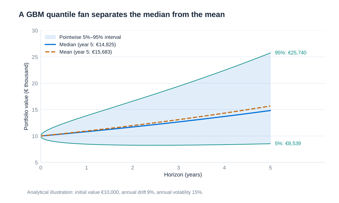
A fan of 5%, 50% and 95% quantiles describes the distribution at each displayed date. It is not a 90% guarantee that an entire path stays inside the band at all intervening dates. Nor is the lowest simulated outcome the maximum possible loss. Distinguishing point-in-time quantiles, path-dependent losses and model uncertainty is essential when communicating risk forecasts to investment clients or decision-makers.
Risk-adjusted performance and incentives
High returns do not by themselves demonstrate skill. A portfolio can earn more because it takes more risk, employs more leverage or accepts an infrequent large loss. Risk-adjusted performance measurement compares reward with the relevant exposure and helps evaluate business units, managers and compensation. The chosen measure must match the decision: total volatility, systematic market risk and capital consumption answer different questions.
Under the capital asset pricing model's assumptions, efficient portfolios combining a risk-free asset and the market portfolio lie on the capital market line:
Here is the risk-free return over the same period, and are the market's expected return and volatility, and is portfolio volatility. The Sharpe ratio measures excess return per unit of total volatility: . With illustrative market return 10%, risk-free return 3% and volatility 20%, it equals . This is an example, not a permanent empirical Sharpe ratio guaranteed by investing in the market.
The security market line instead relates expected return to beta:
It applies in the CAPM to individual securities and portfolios, including inefficient portfolios, because diversifiable risk is not priced in that model. The Treynor ratio divides excess return by beta, . Jensen's alpha measures return above the CAPM benchmark:
Sharpe is appropriate when the investor bears the portfolio's total risk; Treynor and alpha focus on systematic risk and depend on the benchmark model. Treynor becomes difficult to interpret when beta is near zero or negative. Ex-post estimated alpha is uncertain and can reflect an omitted risk factor rather than skill. Comparing ratios also requires consistent horizons, financing assumptions and return definitions.
For a bank business unit, risk-adjusted return on capital, or RAROC, commonly compares risk-adjusted income with allocated economic capital. The numerator should specify the treatment of expected losses, operating costs and taxes; the denominator should identify the capital convention. Comparing RAROC with a required return on capital links performance to shareholder value. Compensation based on this framework can be more informative than a bonus tied only to current profits, but it still requires independent risk measurement, limits, accountability and attention to losses that emerge after the measurement period.