
10. Liquidity Risk
Being valuable is different from being able to pay
Liquidity is the ability to meet obligations when they fall due without incurring unacceptable losses. An institution needs the right amount of cash, in the right currency, in the right legal entity and before the relevant deadline. Assets with substantial long-term value cannot pay today’s creditor unless they can be sold, pledged or otherwise converted into usable funds in time. This is why a profitable business, or even one with assets worth more than its liabilities, can encounter a liquidity crisis.
Funding liquidity risk is the risk of being unable to obtain cash needed for payments, collateral calls or refinancing. Market liquidity risk is the risk that an asset cannot be sold or financed promptly at a price close to its undisturbed value. The two risks interact: an inability to refinance can force an asset sale, while the discount on that sale can worsen the institution’s financial position and undermine creditors’ willingness to lend.
Solvency concerns the capacity of asset value and future earnings to cover liabilities. Liquidity concerns the timing and accessibility of payment resources. The distinction is analytically useful, but crises rarely remain neatly separated. Credit losses can cause lenders to withdraw funding; a funding crisis can then generate fire-sale losses large enough to threaten solvency. Liquidity analysis should therefore incorporate both confidence shocks and deterioration in the underlying business.
How financial institutions produce and consume liquidity
Commercial banks provide customers with liquid deposits while financing assets such as mortgages and business loans that cannot all be realised immediately at their carrying value. They also promise liquidity through credit lines and other commitments. This maturity and liquidity transformation is economically useful, but it requires buffers, diversified funding and credible access to additional resources. A customer’s right to withdraw or draw a facility can become the bank’s cash obligation at an inconvenient moment.
Investment banks and securities dealers provide market liquidity by quoting prices and temporarily holding inventories. They also consume liquidity when they finance those inventories, meet margin calls, underwrite securities or bridge a client’s financing. An underwriting plan may assume that securities will be sold quickly; if demand disappears, the intermediary must finance an unwanted inventory for longer than expected. A securitisation pipeline can similarly leave loans or asset-backed securities on the balance sheet when distribution stops.
Funding diversity must be assessed by economic behaviour, not merely by counting contracts. Several lenders may all withdraw because they use the same collateral standard, credit rating or money-market signal. Geographic diversity does not help much if every funding source depends on the same securitisation market remaining open. Concentration by provider, instrument, currency, maturity and collateral type therefore matters.
Cash-flow gaps and survival horizons
A cash-flow ladder assigns expected receipts and payments to time buckets. For bucket , let be cash inflows, cash outflows and the net gap. With initially available cash , the projected balance before additional financing is:
All terms must use the same currency and units. Contractual maturity is the starting point, but behavioural assumptions are necessary for deposits, early repayments, option exercise and facility drawdowns. An expected refinancing is not equivalent to cash already available, particularly under stress. Intraday settlement obligations may require a finer time grid than a daily or weekly forecast.
| Time bucket | Inflows | Outflows | Net gap | Projected cash before new financing |
|---|---|---|---|---|
| Days 1–7 | 20 | 30 | −10 | 15 |
| Days 8–14 | 15 | 35 | −20 | −5 |
| Days 15–30 | 40 | 20 | 20 | 15 |
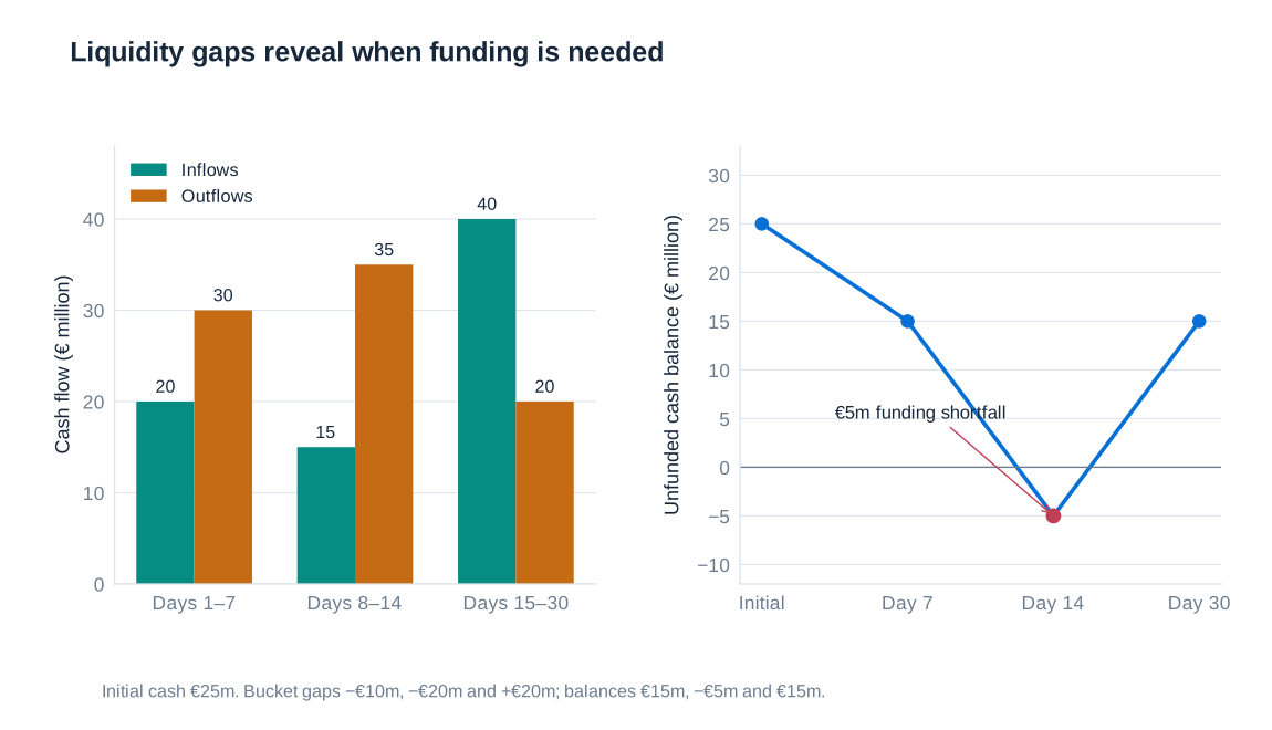
The end-of-month balance is positive, yet the institution has an unfunded €5 million gap by day 14. It needs at least that amount of additional accessible funding by the relevant payment dates; a prudent plan would also allow for uncertainty and any minimum operating cash requirement. The later €40 million inflow cannot retrospectively settle an earlier missed payment. A negative projected balance is a signal that the assumed plan is infeasible without intervention, not a literal balance that can be spent.
A survival horizon identifies how long the institution can continue meeting payments under a specified stress using resources that remain available. It is conditional on assumptions about deposit runoff, collateral haircuts, asset-sale capacity and committed facilities. Stress tests should combine institution-specific pressures with market-wide disruption, because the same event can reduce inflows, increase outflows and make asset sales more expensive.
Measuring market liquidity and collateral capacity
A narrow bid–ask spread indicates a small quoted transaction cost for a specified trade size. Market depth describes how much can be traded without moving the price substantially. Resilience describes how quickly the market absorbs an order imbalance and recovers. Trading volume is useful context, but heavy volume during distressed selling does not necessarily indicate that a large position can be sold cheaply. Executable prices, settlement constraints and the institution’s own position size matter.
Secured funding converts collateral into borrowing capacity. If collateral has market value and the lender applies haircut , a simplified borrowing limit is . The haircut is the fraction of collateral value excluded from the advance. It is not a general definition of the borrower’s accounting equity, although the unfunded part of the position must be financed through other resources.
Consider an explicitly hypothetical repo position. Collateral worth €100 million with a 10% haircut supports €90 million of borrowing. After its price falls to €95 million and the haircut rises to 25%, borrowing capacity becomes:
The borrower must find €18.75 million to repay funding or provide acceptable additional collateral, ignoring interest and other contractual details. This cash requirement is much larger than the €5 million asset-price decline. If the position initially contained €10 million of the borrower’s own funds and no other exposures, its remaining economic equity would still be €5 million before liquidation costs. Positive equity therefore does not by itself solve the immediate funding problem.
Liquidity spirals and the limits of short-term financing
A liquidity spiral arises when worsening market and funding conditions reinforce each other. Lower collateral prices reduce borrowing capacity; larger haircuts intensify the shortfall; borrowers sell assets to raise cash; selling pressure lowers prices further. Dealers facing the same constraints may reduce their capacity to absorb sales. Individually rational attempts to preserve liquidity can therefore worsen conditions for the system as a whole.
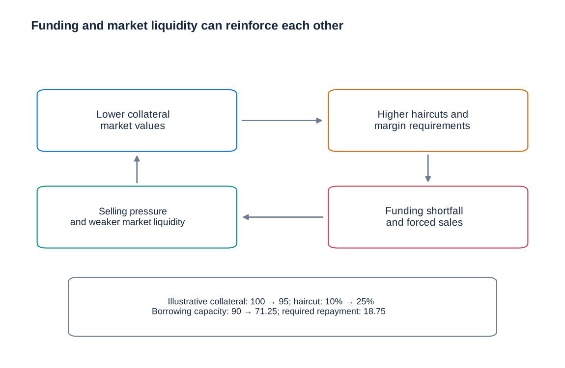
Brunnermeier and Pedersen’s analysis of market and funding liquidity formalises this interaction. The practical implication is that a haircut and an asset price should not always be stressed independently: both may deteriorate together. Collateral that seemed ample in normal markets may support much less borrowing when financing is most needed.
Lehman Brothers illustrates the vulnerability associated with substantial short-term secured funding and confidence-sensitive counterparties. Overnight or very short refinancing makes the institution repeatedly dependent on a fresh lending decision. Its failure cannot be reduced to one haircut or one liquidity mechanism: asset quality, leverage, valuation uncertainty, solvency concerns and counterparty confidence interacted. The general lesson is that a funding plan dependent on uninterrupted rollover needs severe tests of market closure and collateral deterioration.
Northern Rock: wholesale disruption and a retail run
Northern Rock’s 2007 experience shows why the visible queue outside a bank is not necessarily the beginning of the funding problem. Its mortgage business relied heavily on wholesale funding and securitisation. When those markets became difficult to access, the bank sought central-bank liquidity support. Retail withdrawals then intensified the pressure after the support became public.

A depositor who believes others will withdraw may want to withdraw first, because a bank cannot immediately convert its entire loan portfolio into cash without loss. This coordination problem can amplify concerns about a bank even when the initial disturbance comes from wholesale markets. Deposit protection, credible public communication and access to liquidity can influence that behaviour, but none substitutes for a funding structure able to withstand disruption.
The case also illustrates the difference between a solvent asset portfolio under orderly collection and the resources needed to meet rapid withdrawals. On 14 September 2007, the Bank of England announced a support facility against appropriate collateral at a premium interest rate. Analysing the episode requires attention to the wholesale funding model and the subsequent retail run together, rather than treating the photograph of depositors as a complete explanation.
Historical sources: the Bank of England’s Northern Rock liquidity-support announcement and the UK Treasury Committee’s inquiry into the bank’s funding model. The feedback mechanism is developed in Markus K. Brunnermeier and Lasse Heje Pedersen (2009), Market Liquidity and Funding Liquidity.
Contingent funding: IKB and AIG
Liquidity commitments can transmit stress from an apparently separate vehicle to its sponsoring bank. IKB’s involvement with the Rhineland Funding conduit illustrates the mechanism. The vehicle financed longer-lived asset-backed exposures using short-term asset-backed commercial paper. If investors refused to roll that paper, a committed liquidity facility could be drawn, transferring an immediate funding requirement to the bank.
The commitment resembles a contingent promise to absorb assets or provide cash when market financing becomes unavailable. The analogy to a written put is useful because the obligation tends to become costly in adverse states. It is not an assertion that every liquidity facility has the same payoff as a simple traded put: draw conditions, collateral eligibility, credit exclusions and recourse depend on the actual contract. Exposure analysis must read those terms and consider correlated drawdowns across facilities.
AIG provides a related but distinct mechanism. Credit protection sold on structured-credit exposures created obligations that depended on collateral agreements as well as eventual credit events. Falling valuations and rating-related triggers could generate collateral calls before the reference assets suffered final default losses. Cash therefore became necessary on a timetable different from the eventual insurance or credit-loss settlement.
This distinction prevents two errors. A margin call does not by itself establish the ultimate loss on the underlying asset, but neither can it be dismissed merely because that loss has not yet occurred. Counterparty agreements, downgrade provisions, eligible collateral and the ability to obtain cash must be incorporated into stress tests. A position described as remote from expected default can still have demanding liquidity consequences.
Pension hedges and the 2022 gilt-market disruption
Liability-driven investment seeks to manage the sensitivity of pension assets relative to promised benefits. A pension liability resembles a stream of long-dated payments, so its present value generally rises when discount rates fall. Receiving a fixed rate and paying a floating rate in an interest-rate swap can add asset-side interest-rate sensitivity and help hedge that liability exposure without buying the full notional amount of bonds.
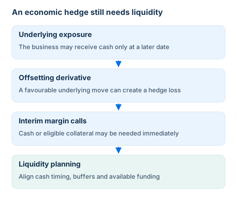
For a hypothetical illustration, take a scheme with £100 million of liabilities, £20 million in gilts and £80 million in illiquid private-equity investments. Suppose it also enters a receive-fixed, pay-floating swap with £80 million notional. The swap notional is a reference amount for payments and sensitivity; it is not an additional £80 million asset to add to the balance sheet. At inception, a market-rate swap can have approximately zero value.
If yields rise sharply, the gilts and the receive-fixed swap lose value. The present value of pension liabilities can fall too, so the scheme’s long-run funding position need not deteriorate in the same way as its immediate cash position. The lower liability valuation, however, delivers no cash with which to meet the swap’s collateral call. Private-equity holdings may not be saleable quickly, leaving gilts or other liquid assets as the immediate source of funds.
During the September 2022 UK gilt-market disruption, distressed selling by liability-driven investment funds reinforced falling prices and collateral pressure. The Bank of England introduced temporary, targeted gilt purchases to restore market functioning and allow time for adjustment. The case demonstrates that a hedge of long-term liability value needs a separately funded collateral buffer. The asset allocation and numbers above explain the mechanism; they are not a reconstruction of every affected fund.
The historical mechanism and intervention are described by the Bank of England in Financial stability buy/sell tools: a gilt market case study (2023).
Metallgesellschaft: a long-term hedge with short-term cash demands
Metallgesellschaft’s 1993 difficulties illustrate a similar timing problem in commodity markets. Long-term commitments to deliver oil products at fixed prices created exposure to rising oil prices. Long positions in shorter-dated oil futures could offset part of that exposure: higher oil prices would increase the cost of supplying customers but generate gains on the futures.
When oil prices fell, the futures generated losses and cash margin requirements. The fixed-price delivery commitments became economically more favourable, but that benefit was embedded in future deliveries rather than immediately available cash. Maintaining the hedge therefore required financing the interval between derivative losses and the realisation of offsetting operating benefits.
A one-for-one match in barrel quantities is not automatically a perfect hedge. Futures maturity, the shape of the forward curve, roll costs, product quality, customer performance and the timing of deliveries all matter. The case should consequently not be interpreted as proof that an otherwise riskless strategy failed solely because managers misunderstood margin. Its broader lesson is that economic hedging, basis risk and the funding of intermediate cash flows must be evaluated jointly.
Central-bank access and foreign-currency liquidity
Central-bank funding is conditional on eligible counterparties, acceptable collateral and the governing operational rules. In February 2015, the ECB removed the waiver that had allowed certain Greek sovereign-issued or guaranteed instruments to serve as collateral despite not meeting normal minimum credit-rating requirements. This did not remove Greek banks’ counterparty status or mean that every channel of central-bank support ceased. The ECB explained that relevant national-central-bank emergency liquidity assistance could address needs within the applicable rules.
The distinction matters for a contingency plan. An asset may retain economic value while becoming ineligible in a particular facility. Funding capacity then changes even without an immediate contractual default. Available collateral, operational readiness and the conditions attached to alternative facilities should be mapped in advance; emergency assistance must not be modelled as unconditional private funding.
Currency creates another constraint. A European bank holding dollar assets cannot necessarily finance a dollar payment with euro cash at an acceptable cost during a dollar shortage. It may depend on dollar wholesale borrowing or on rolling foreign-exchange swaps. Those channels introduce refinancing and cross-currency basis risk, even where the long-term currency exposure is hedged.
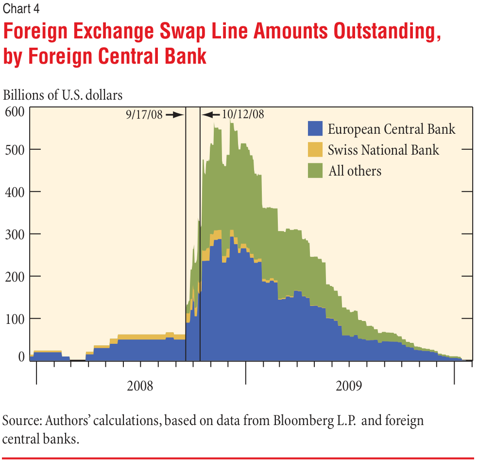
Central-bank swap lines address this currency-specific shortage by enabling a foreign central bank to obtain dollars from the Federal Reserve and provide dollar liquidity in its jurisdiction. The historical expansion of such arrangements during the financial crisis reflects strains in international dollar funding. The figure records that historical episode; it should not be read as a forecast or as a statement that every institution has direct access to the Federal Reserve.
Primary sources: ECB, Eligibility of Greek bonds used as collateral in Eurosystem monetary policy operations (4 February 2015), Federal Reserve, Central bank liquidity swaps; and Michael J. Fleming and Nicholas J. Klagge (2010), The Federal Reserve’s Foreign Exchange Swap Lines, Chart 4.
The Liquidity Coverage Ratio and a usable stress buffer
The Basel Liquidity Coverage Ratio, or LCR, compares a stock of qualifying high-quality liquid assets with net cash outflows in a specified 30-calendar-day stress scenario. Under normal conditions, the minimum ratio is 100%:
Here HQLA is the eligible liquid-asset stock after applicable adjustments, and is stressed net outflow over 30 days. The buffer is intended to be used during stress. Basel explicitly allows the ratio to fall below 100% in such circumstances, with supervisory assessment and response reflecting the situation. Treating every stress-time use of the buffer as automatically impermissible would undermine its purpose.
HQLA must meet asset-quality and operational conditions, including availability for monetisation. Nominal ownership is insufficient if an asset is encumbered or cannot be mobilised by the liquidity-management function. Level 1 assets face no overall composition cap; Level 2 assets are limited to 40% of the qualifying stock, and Level 2B assets to 15%, subject to the framework’s adjustments. The relevant haircuts and caps mean that the accounting value of securities is not necessarily their HQLA amount.
Stressed outflows apply prescribed assumptions to funding withdrawals, commitments and other obligations. Eligible inflows are restricted, including an overall cap of 75% of outflows in the basic calculation. If is stressed outflow and eligible inflow before that cap, the simplified expression is:
Consider a hypothetical bank with €120 million of eligible HQLA, €160 million of stressed outflows and €60 million of eligible inflows. The cap is €120 million, so all €60 million of inflows are counted. Net outflows are €100 million and the LCR is , or 120%. The €20 million excess is a buffer above this particular regulatory requirement, not proof that every payment path or stress is covered.
If eligible inflows instead equal €140 million while outflows remain €160 million, the cap permits only €120 million to offset outflows. Net outflows are therefore €40 million rather than €20 million. The cap limits reliance on expected receipts and ensures a minimum holding of liquid resources relative to gross stressed outflows.
Regulatory sources: Basel Framework LCR20 on the minimum and stress-time buffer use, LCR30 on HQLA, and LCR40 on cash flows. Basel standards provide the international framework; jurisdictional implementation and institution-specific requirements must also be considered.
The Net Stable Funding Ratio
The Net Stable Funding Ratio, or NSFR, addresses the stability of the funding structure over a one-year horizon. It compares available stable funding, ASF, with required stable funding, RSF. Funding categories receive weights reflecting their expected stability; assets and selected off-balance-sheet exposures receive weights reflecting their funding needs:
Here denotes a funding amount, including eligible capital; is its ASF factor. The amount and factor describe an asset category, while captures relevant off-balance-sheet requirements. The factors are regulatory weights, not forecasts that an identical fraction will certainly leave or remain. The NSFR is a structural measure and does not replace a dated cash forecast.
| ASF factor | Representative qualifying funding |
|---|---|
| 100% | Eligible regulatory capital and qualifying funding with effective residual maturity of at least one year |
| 95% | Qualifying stable retail and small-business demand deposits or deposits with residual maturity below one year |
| 90% | Corresponding less stable retail and small-business deposits |
| 50% | Non-financial corporate funding below one year; certain other funding from six months to below one year |
| 0% | Funding outside the qualifying categories, including ordinary very short-term financial-institution funding |
Deposit classification matters: the 95% and 90% factors are distinct from the lower weights in early versions of the international liquidity proposals. “Stable” is a defined regulatory category, not an informal judgement that a customer seems loyal. Effective maturity, early-withdrawal rights and the identity of the provider can affect classification.
| RSF factor | Representative qualifying asset or exposure |
|---|---|
| 0% | Cash and central-bank reserves |
| 5% | Unencumbered Level 1 assets other than cash and central-bank reserves |
| 10% | Qualifying financial-institution loans below six months, secured by reusable Level 1 collateral |
| 15% | Unencumbered Level 2A assets and certain other financial-institution loans below six months |
| 50% | Unencumbered Level 2B assets and qualifying shorter-term non-financial loans |
| 65% | Qualifying unencumbered residential mortgages of at least one year with standardised risk weight no greater than 35% |
| 85% | Other qualifying performing long-term non-financial loans; physical commodities including gold; derivative initial margin |
| 100% | Fixed assets, non-performing loans and assets encumbered for at least one year |
| 5% of undrawn amount | Irrevocable and conditionally revocable credit and liquidity facilities |
The tables give representative categories, not a complete substitute for the rules. A short maturity alone does not give every loan a zero RSF factor. Encumbrance, counterparty type and derivative treatment can change the requirement. Undrawn commitments also matter because they can require funding after a customer exercises the right to draw.
For a hypothetical €100 million balance sheet, suppose assets consist of €10 million cash, €20 million qualifying unencumbered Level 1 securities and €70 million qualifying mortgages in the 65% category. Funding consists of €10 million eligible capital, €50 million stable qualifying deposits in the 95% category and €40 million ordinary financial-institution borrowing with maturity below six months and a 0% factor. Ignoring other exposures:
Both assets and funding total €100 million, but the weighted amounts differ. Passing the ratio does not eliminate the need to refinance the €40 million borrowing or meet deposit withdrawals. The example demonstrates the distinction between a structural regulatory test and a complete survival analysis.
Regulatory sources: Basel Framework NSF20 on the ratio, NSF30 on ASF and RSF definitions, and NSF99 for category summaries.
Turning measurements into a contingency funding plan
The LCR examines a specified short stress, while the NSFR disciplines structural funding. A bank can satisfy both and remain exposed to a concentrated payment, an unavailable currency, an operational barrier or a shock beyond their assumptions. Internal cash ladders, collateral inventories and stress tests should therefore supplement regulatory ratios.
A contingency plan connects observable warning signals to actions that can actually be executed. Signals can include rapid deposit outflows, widening funding spreads, larger haircuts, rating changes and declining collateral capacity. Responses might involve drawing genuinely available committed lines, mobilising prepositioned collateral, obtaining longer funding, reducing positions or slowing new commitments. Each action needs an owner, a realistic execution time and an estimate of its effect on counterparties and markets.
Plans must avoid double counting. The same security cannot simultaneously fund an asset sale and remain pledged to support existing borrowing. A facility cannot be treated as unconditional if a covenant or adverse-change clause could prevent drawing. Transfers between subsidiaries may face legal or operational barriers, and an assumed sale price must reflect the size of the position under stress.
Liquidity risk management ultimately combines balance-sheet design with preparation for adverse timing. It asks how a business model supplies liquidity to others, when those promises become cash obligations, and which resources remain usable when confidence falls. Economic hedges, accounting profit and regulatory compliance all contribute information, but the decisive operational question remains whether every due payment can be funded on time.