
7. Credit Risk: Measurement, Ratings and Portfolio Management
Credit risk arises whenever one party depends on another party to honour an obligation. A bank's loan book is the obvious example, but the same exposure appears in trade receivables, credit cards, leasing, instalment purchases and derivatives. A traveller who pays for an airline ticket before departure extends credit to the airline; a telecommunications provider that supplies a handset before collecting all monthly payments extends credit to the customer. Bond investors, landlords and suppliers therefore face different versions of the same problem: promised cash flows may arrive late, arrive only partly or never arrive.
Default, deterioration and the definition of loss
A default can involve insolvency, a material payment that remains overdue, or a distressed restructuring that reduces the creditor's economic claim. Regulatory definitions also consider whether the borrower is unlikely to pay without enforcement of collateral. A 90-day past-due trigger is widely used, but its precise application depends on the applicable framework, materiality thresholds and exposure category. Legal bankruptcy is consequently neither the only default event nor a necessary condition for every credit loss. A rating of D or a non-performing-loan designation communicates a default-related status, whereas a performing loan can already have substantial credit risk.
Credit deterioration matters before default. A rating downgrade, an increase in an internally estimated probability of default or a widening market credit spread can reduce the present value of a claim while all payments remain current. Default risk, migration risk and spread risk overlap economically but are not interchangeable measurement categories. A trading portfolio may recognise spread changes through market-risk measures, while a banking-book portfolio uses default and impairment measures. Calling an exposure “credit risk” does not by itself determine its accounting treatment or its prudential classification.
Measurement must therefore specify the horizon, valuation basis and aggregation level. The eventual unpaid amount on one loan is different from the present market-value loss on a bond, and neither is the same as the unexpected loss of a diversified portfolio. Internal ratings and external ratings describe credit quality; expected loss describes a mean monetary shortfall; economic capital describes a tail buffer; and risk-weighted assets are a regulatory denominator used to determine capital requirements. Treating these quantities as substitutes obscures the decision each one supports.
PD, LGD and EAD
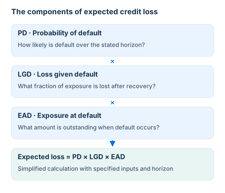
The three central components are probability of default, or PD; exposure at default, or EAD; and loss given default, or LGD. PD is the probability that a specified default event occurs over a specified horizon. EAD is the amount exposed when default occurs, including relevant drawings or accrued amounts rather than necessarily today's outstanding principal. LGD is the fraction of that exposure lost after allowing for recoveries and the associated costs and timing. If recovery is immediate, costless and measured on the same exposure basis, LGD equals one minus the recovery rate.
For deterministic EAD and an appropriately defined conditional mean LGD, the familiar one-period relation is
PD and LGD enter as decimals, and EAD is a currency amount, so expected loss has the same currency unit. Consider a €100 loan with a 10% probability of default and an expected recovery of €50 if default occurs. The conditional loss is €50, LGD is 50%, and expected loss is euros. The borrower does not pay an “expected” €5 loss in every outcome: the simplified distribution has a €50 loss with probability 10% and no loss with probability 90%.
| Outcome | Probability | Credit loss | Contribution to expected loss |
|---|---|---|---|
| No default | 90% | €0 | €0 |
| Default with €50 recovery | 10% | €50 | €5 |
| Total | 100% | Outcome-dependent | €5 |
The factorisation needs care when exposure and recovery are random. With a default indicator , the general object is , not automatically . A borrower may draw unused credit immediately before default, while collateral values fall during the same downturn. A revolving facility with €60 drawn and €40 undrawn, for example, has EAD of €80 if the assumed conversion factor on the undrawn portion is 50%. That is a modelling assumption, not a universal conversion factor. Legal enforceability, collateral liquidity and recovery costs can make LGD materially higher than the apparent shortfall between loan principal and today's collateral valuation.
For a multi-year exposure, losses at different dates and in different economic scenarios must be combined without counting the same default repeatedly. Let be the marginal probability of first default in year under scenario , the scenario probability and a discount factor consistent with the measurement purpose. A simplified representation is
The scenario weights sum to one. The loss severity should incorporate the timing of recoveries consistently, so discounting is not applied twice. Accounting expected credit loss, a market price and prudential expected loss can use different probability concepts, horizons and prescribed inputs. Sharing the labels PD, LGD and EAD does not make the resulting estimates identical.
Impairment, write-offs and fair-value losses
Under the general IFRS 9 impairment model, Stage 1 ordinarily recognises 12-month expected credit losses. This is the lifetime cash shortfall associated with defaults that could occur in the next 12 months, not merely cash payments missed during those months. A significant increase in credit risk moves an exposure to Stage 2 and lifetime expected credit losses. Stage 3 concerns credit-impaired assets and also uses lifetime expected losses; interest revenue is generally calculated on the net carrying amount. Special approaches and exceptions exist, so these three stages describe the general model rather than every financial asset.
An impairment charge changes the allowance and profit or loss; it does not necessarily mean that the borrower has already defaulted. A write-off directly reduces the gross carrying amount when there is no reasonable expectation of recovering all or part of the asset. It need not wait for the formal end of insolvency proceedings. If the loss was already fully provided for, the later write-off mainly uses the existing allowance rather than creating the same expense a second time. Changes in fair value are a separate channel for instruments measured at fair value.
The US current expected credit losses model, CECL, belongs to US GAAP and is not another name for IFRS 9. For financial assets within its amortised-cost scope, it generally recognises lifetime expected credit losses from initial recognition. Both systems are forward-looking, but their recognition frameworks differ. Comparing banks across accounting systems therefore requires more than comparing the words “expected loss” in their reports.
Accounting references: ESRB comparison of European and US expected-loss approaches; IFRS 9 impairment review, including write-offs; Federal Reserve CECL guidance.
Expected loss, unexpected loss and economic capital
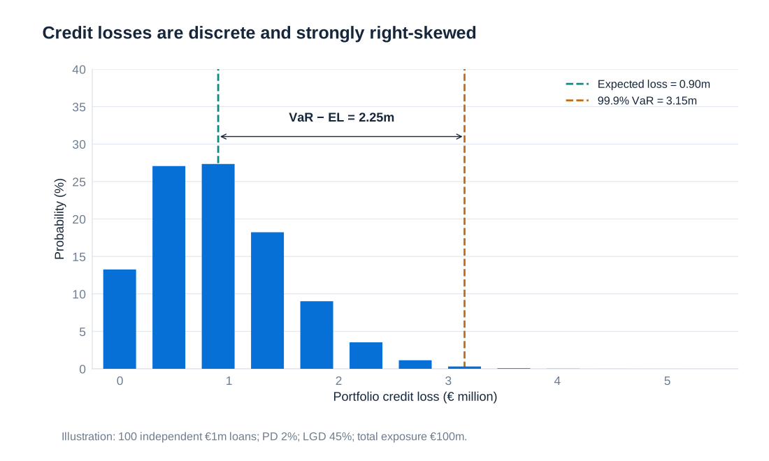
At portfolio level, loss is a random variable . Its mean describes expected loss; a quantile describes a tail outcome. Define as the smallest loss level reached with cumulative probability at least . One common economic-capital convention is , the tail loss above the mean. In this manual, unexpected loss is the standard deviation . Some institutions use that term for quantile-minus-mean instead; stating the convention is essential because these quantities differ.
Expected credit losses are ordinarily considered in pricing, provisions and operating income. Capital provides capacity to absorb adverse deviations and other risks. The economic-capital confidence level is a management choice linked to the institution's solvency objective; 99%, 99.9% and 99.98% are not interchangeable universal standards. Regulatory capital is determined by a separate set of rules. Risk-weighted assets, or RWA, are neither cash losses nor capital itself: a capital ratio applies a required percentage to the RWA denominator.
Consider an illustrative portfolio of 100 independent loans, each with EAD €1 million, one-year PD 2% and deterministic LGD 45%. The number of defaults is binomial with parameters 100 and 0.02, and total loss is million euros. Expected loss is €0.9 million. The standard deviation is million euros. The exact 99.9% loss quantile is seven defaults, or €3.15 million; economic capital is therefore €3.15 million minus €0.9 million, giving €2.25 million. The quantile is determined from the binomial cumulative distribution, not a normal approximation. This stylised example isolates diversification across independent borrowers; real portfolios can have much more severe tails because defaults are dependent.
Credit risk frequently dominates banks' risk allocations, but the share depends on business model and measurement basis. Historical illustrations report credit risk as 49.6% of €77 billion of economic capital for five large German banks, with approximately €38 billion allocated to credit risk; total credit exposure was €1,938 billion and retail and small businesses represented 29.3%. Another historical savings-bank illustration allocates approximately 78% to credit risk, 20% to market risk and 1% to operational risk, with rounding. Such figures illustrate materiality rather than providing a current banking-sector benchmark, and economic-capital allocations must not be relabelled as RWA.
The economic logic of the IRB capital formula
The internal ratings-based approach, IRB, links regulatory credit capital to PD, LGD, EAD, maturity and a prescribed asset-correlation function. Its underlying asymptotic single-factor model assumes a highly granular portfolio: individual borrower shocks diversify, but a common systematic factor remains. A severe state of that factor raises the conditional default rate. For an ordinary non-defaulted corporate exposure, the core expression can be written
Here is the standard normal cumulative distribution function, its inverse, the prescribed asset correlation, effective maturity in years, and a capital ratio before multiplying by EAD. For the basic corporate correlation function, before applicable adjustments,
The square root on the systematic-factor loading is essential. The term is a conditional stressed loss rate; subtracting removes expected loss from the core unexpected-loss component. The factor 12.5 converts capital into RWA at an 8% reference capital ratio. RWA are consequently not equal to the 99.9% portfolio loss quantile. The maturity adjustment changes the charge according to effective maturity; the ordinary framework commonly constrains maturity between one and five years, with specific exceptions. Asset classes, smaller-company adjustments and certain financial-institution exposures require their own prescribed treatment.
The legacy Basel II scaling multiplier 1.06 has been removed from the revised Basel framework. Likewise, the old 0.03% PD floor is not a universal current rule: the revised framework generally uses 0.05% for corporate and bank exposures, with sovereign exceptions and distinct retail provisions. A zero observed default count does not establish zero credit risk. Long-run calibration, data requirements, conservatism and applicable floors address sparse-default samples.
Basel standards are implemented through jurisdiction-specific law. In the EU, CRR3 introduced the final Basel III package from 2025, including an output floor phased from 50% towards 72.5% in 2030. This limits the reduction in aggregate capital requirements obtainable from internal models relative to standardised calculations; it is not a floor on each individual loan's PD. Sovereign exposures are not universally assigned zero risk weight: preferential treatment depends on the applicable approach and conditions, including relevant domestic-currency provisions. Regulatory zero weight would in any event not mean economic impossibility of default.
Prudential references: Basel CRE31 risk-weight functions; CRE32 risk components; removal of the 1.06 multiplier; Regulation (EU) 2024/1623; EU output-floor transition.
Market-implied default probabilities
Credit assessment can use financial statements, management information, payment histories, external ratings and market prices. Bond and CDS prices provide forward-looking information, but they price risk under a risk-neutral measure. A risk-neutral PD is a valuation input that reproduces market prices under appropriate discounting; it is not automatically the physical frequency with which comparable borrowers will default.
Consider one-year zero-coupon bonds with face value €100. The risk-free yield is 5%, giving a price of euros. A risky bond has a promised yield of 10%, giving a price of euros. Suppose its maturity payoff is €100 without default and €50 after default. With risk-neutral default probability ,
The promised 10% yield is not the expected realised return. Risk-neutral expected payoffs discounted at 5% reproduce the price. The physical PD may be lower when investors require compensation for systematic default risk, but there is no universal fixed difference between the two probabilities. Liquidity, risk aversion, taxes, contractual features and market frictions can also affect spreads, so a simple spread-to-PD conversion can misattribute non-default components to default risk.
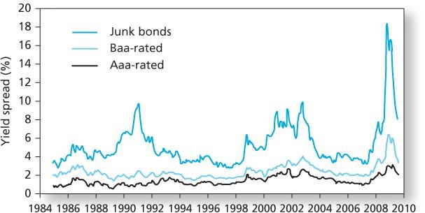
Historical bond spreads widen markedly in downturns, especially for speculative-grade debt. That movement can reflect worse expected cash flows, lower recovery prospects, a higher price of bearing risk and deteriorating market liquidity at the same time. A widening spread is therefore a warning signal, not a direct observation of a uniquely identified physical PD.
Structural credit risk: the Merton model
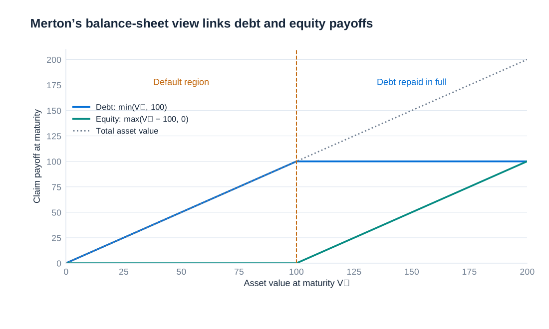
A structural model connects default to the value of the borrower's assets. In the simplest Merton setting, the firm has asset value and one zero-coupon debt obligation with face value due at time . Default occurs at maturity when . With limited liability, equity receives , so equity is a call option on the firm's assets. Debt receives , equivalently a risk-free payment of minus a put-option payoff.
Under risk-neutral geometric Brownian motion, constant asset volatility , a constant continuously compounded risk-free rate and no asset payouts, equity value is
The physical default probability replaces the risk-neutral drift with the physical expected asset return in the distance-to-default expression. Higher leverage reduces the distance between asset value and the debt threshold; higher asset volatility increases exposure to downside states. Because corporate assets are not usually traded directly, implementation must infer asset value and volatility from observed securities and balance-sheet information. The assumption of default only at a single maturity is restrictive: real firms have several debt maturities, covenants, liquidity constraints and possible early default.
Structural models and statistical accounting-score models should not be confused. A market-based expected-default-frequency approach can use structural intuition and empirical calibration, while a private-firm score based on accounting ratios estimates risk statistically. The product name or the rating provider does not establish which model is being used. The relevant questions are its inputs, target event, horizon, probability measure and validation performance.
External ratings and their meaning
External ratings order issuers or obligations by creditworthiness. The investment-grade boundary is BBB− for S&P and Fitch and Baa3 for Moody's; lower categories are speculative grade. A notch is one step within this ordered scale. An issuer rating and an issue rating can differ because a particular claim has collateral, guarantees or subordination. Rating symbols also have agency-specific definitions; a cross-agency correspondence is a broad comparison, not a guarantee that the underlying risks or methodologies are identical.
| S&P | Fitch | Moody’s | Broad category |
|---|---|---|---|
| AAA | AAA | Aaa | Investment grade |
| AA+ | AA+ | Aa1 | Investment grade |
| AA | AA | Aa2 | Investment grade |
| AA− | AA− | Aa3 | Investment grade |
| A+ | A+ | A1 | Investment grade |
| A | A | A2 | Investment grade |
| A− | A− | A3 | Investment grade |
| BBB+ | BBB+ | Baa1 | Investment grade |
| BBB | BBB | Baa2 | Investment grade |
| BBB− | BBB− | Baa3 | Investment grade |
| BB+ | BB+ | Ba1 | Speculative grade |
| BB | BB | Ba2 | Speculative grade |
| BB− | BB− | Ba3 | Speculative grade |
| B+ | B+ | B1 | Speculative grade |
| B | B | B2 | Speculative grade |
| B− | B− | B3 | Speculative grade |
| CCC+ | CCC+ | Caa1 | Speculative grade |
| CCC | CCC | Caa2 | Speculative grade |
| CCC− | CCC− | Caa3 | Speculative grade |
| CC | CC | Ca | Speculative grade |
| C | C | C | Speculative grade |
At the bottom of the scale, S&P uses default-related designations including D and SD, and Fitch distinguishes D and RD. Moody's does not use D as an ordinary long-term rating category; its C category can include obligations in default. Rating methodologies also differ in the relative emphasis placed on default likelihood, loss severity and the credit characteristics of particular obligations. “Through the cycle” describes an effort to look beyond temporary conditions, not a promise that a rating never changes during a cycle or corresponds to one permanently fixed one-year PD.
From business and financial risk to an anchor rating
A corporate rating combines business risk with financial risk. Business risk reflects country and industry conditions and the firm's competitive position. Financial risk draws on cash generation, debt burden and coverage ratios after accounting adjustments that improve comparability. An initial anchor is then modified for diversification, capital structure, financial policy, liquidity, management and governance, and comparable-rating analysis. Group or government support can change the final issuer assessment relative to the stand-alone credit profile.
In the historical process example, country risk is scored 2 (low), industry risk 4 (moderately high), their combined country-and-industry assessment is 4, and competitive position is 3 (satisfactory). The resulting business-risk profile is 3 (satisfactory). These are category scores within that methodology, not probabilities or quantities to average mechanically. The financial assessment and later modifiers are still needed before determining an issuer rating.
A historical Daimler illustration shows why reported debt is not necessarily the debt figure used in credit analysis. Operating leases and post-retirement obligations increase adjusted obligations, while surplus cash and financing-business adjustments can reduce the industrial debt measure. The following historical figures are in EUR millions. A denotes actual data; P and E denote projected or estimated columns. Repeated projected values are retained as stated, not interpreted as realised later outcomes.
| Adjustment | 2012A | 2013A | 2014P | 2015E | 2016E |
|---|---|---|---|---|---|
| Reported debt | 76,251 | 77,738 | 77,738 | 77,738 | 77,738 |
| Operating leases | 1,672 | 1,501 | 1,501 | 1,501 | 1,501 |
| Post-retirement benefit obligations | 10,324 | 9,109 | 9,109 | 9,109 | 9,109 |
| Less surplus cash | −12,837 | −13,848 | −13,848 | −13,848 | −13,848 |
| Less captive-finance adjustment | −64,272 | −67,497 | −67,497 | −67,497 | −67,497 |
| Other adjustments | 120 | 454 | 454 | 454 | 454 |
| Fully adjusted debt | 11,258 | 7,457 | 7,457 | 7,457 | 7,457 |
The adjusted debt amount is approximately €11,258 million for 2012 and €7,457 million for the later columns. Small reconciliation differences can arise from the rounding of the individual displayed adjustments. The accounting perimeter matters: separating captive finance debt from industrial debt does not make those finance-company obligations disappear from the consolidated group or remove their economic risks.
The next historical grid translates ratios into financial-risk categories. FFO is funds from operations, EBITDA is earnings before interest, tax, depreciation and amortisation, OCF is operating cash flow, FOCF is free operating cash flow, and DCF here means discretionary cash flow, not discounted cash flow. The ratios are agency-adjusted measures. Thresholds depend on methodology and industry; this 2014-era grid explains the rating process and is not a current universal rulebook.
| Financial risk | FFO/debt (%) | Debt/EBITDA (×) | FFO/cash interest (×) | EBITDA/interest (×) | OCF/debt (%) | FOCF/debt (%) | DCF/debt (%) |
|---|---|---|---|---|---|---|---|
| Minimal | >60 | <1.5 | >13 | >15 | >50 | >40 | >25 |
| Modest | 45–60 | 1.5–2 | 9–13 | 10–15 | 35–50 | 25–40 | 15–25 |
| Intermediate | 30–45 | 2–3 | 6–9 | 6–10 | 25–35 | 15–25 | 10–15 |
| Significant | 20–30 | 3–4 | 4–6 | 3–6 | 15–25 | 10–15 | 5–10 |
| Aggressive | 12–20 | 4–5 | 2–4 | 2–3 | 10–15 | 5–10 | 2–5 |
| Highly leveraged | <12 | >5 | <2 | <2 | <10 | <5 | <2 |
Combining business and financial assessments gives the following historical anchor matrix. Lower-case symbols identify intermediate analytical anchors. A satisfactory business profile with minimal financial risk produces an a/a− anchor in this example; weak liquidity or an aggressive financial policy can still alter the eventual rating. A matrix cannot substitute for assessment of the definitions underlying its rows and columns.
| Business risk | Minimal | Modest | Intermediate | Significant | Aggressive | Highly leveraged |
|---|---|---|---|---|---|---|
| Excellent | aaa/aa+ | aa | a+/a | a− | bbb | bbb−/bb+ |
| Strong | aa/aa− | a+/a | a−/bbb+ | bbb | bb+ | bb |
| Satisfactory | a/a− | bbb+ | bbb/bbb− | bbb−/bb+ | bb | b+ |
| Fair | bbb/bbb− | bbb− | bb+ | bb | bb− | b |
| Weak | bb+ | bb+ | bb | bb− | b+ | b/b− |
| Vulnerable | bb− | bb− | bb−/b+ | b+ | b | b− |
Default probabilities across horizons
A rating becomes more useful for measurement when it is connected to a clearly defined default frequency and horizon. The historical table below reports average cumulative corporate default rates by initial rating, measured in percent, over the 1981–2014 observation period. A cumulative rate includes defaults occurring at any time before the stated horizon. The rows are historical averages for different initial-rating cohorts; they are not forecasts for a current issuer and should not be combined as though every category had the same number of observations.
| Initial rating | 1 year | 2 years | 3 years | 4 years | 5 years | 6 years | 7 years | 8 years | 9 years | 10 years | 11 years | 12 years | 13 years | 14 years | 15 years |
|---|---|---|---|---|---|---|---|---|---|---|---|---|---|---|---|
| AAA | 0.00 | 0.03 | 0.14 | 0.24 | 0.36 | 0.47 | 0.53 | 0.61 | 0.67 | 0.74 | 0.77 | 0.80 | 0.84 | 0.91 | 0.98 |
| AA | 0.02 | 0.07 | 0.13 | 0.24 | 0.35 | 0.46 | 0.56 | 0.65 | 0.73 | 0.82 | 0.90 | 0.97 | 1.05 | 1.12 | 1.19 |
| A | 0.07 | 0.16 | 0.27 | 0.41 | 0.57 | 0.75 | 0.95 | 1.13 | 1.32 | 1.51 | 1.69 | 1.84 | 2.00 | 2.15 | 2.32 |
| BBB | 0.20 | 0.57 | 0.96 | 1.46 | 1.95 | 2.43 | 2.84 | 3.26 | 3.66 | 4.06 | 4.49 | 4.84 | 5.17 | 5.50 | 5.84 |
| BB | 0.76 | 2.35 | 4.23 | 6.06 | 7.71 | 9.28 | 10.59 | 11.75 | 12.80 | 13.74 | 14.52 | 15.18 | 15.75 | 16.24 | 16.77 |
| B | 3.88 | 8.80 | 12.97 | 16.22 | 18.70 | 20.72 | 22.37 | 23.69 | 24.82 | 25.91 | 26.82 | 27.57 | 28.26 | 28.88 | 29.49 |
| CCC/C | 26.38 | 35.58 | 40.67 | 43.77 | 46.28 | 47.24 | 48.27 | 49.06 | 50.03 | 50.73 | 51.28 | 51.94 | 52.72 | 53.38 | 53.38 |
| Investment grade | 0.11 | 0.29 | 0.50 | 0.76 | 1.03 | 1.29 | 1.54 | 1.78 | 2.01 | 2.24 | 2.46 | 2.65 | 2.83 | 3.01 | 3.20 |
| Speculative grade | 3.87 | 7.58 | 10.79 | 13.39 | 15.49 | 17.23 | 18.69 | 19.90 | 20.98 | 21.97 | 22.79 | 23.49 | 24.13 | 24.68 | 25.22 |
| All rated | 1.50 | 2.95 | 4.23 | 5.31 | 6.20 | 6.97 | 7.62 | 8.18 | 8.68 | 9.15 | 9.56 | 9.90 | 10.21 | 10.49 | 10.78 |
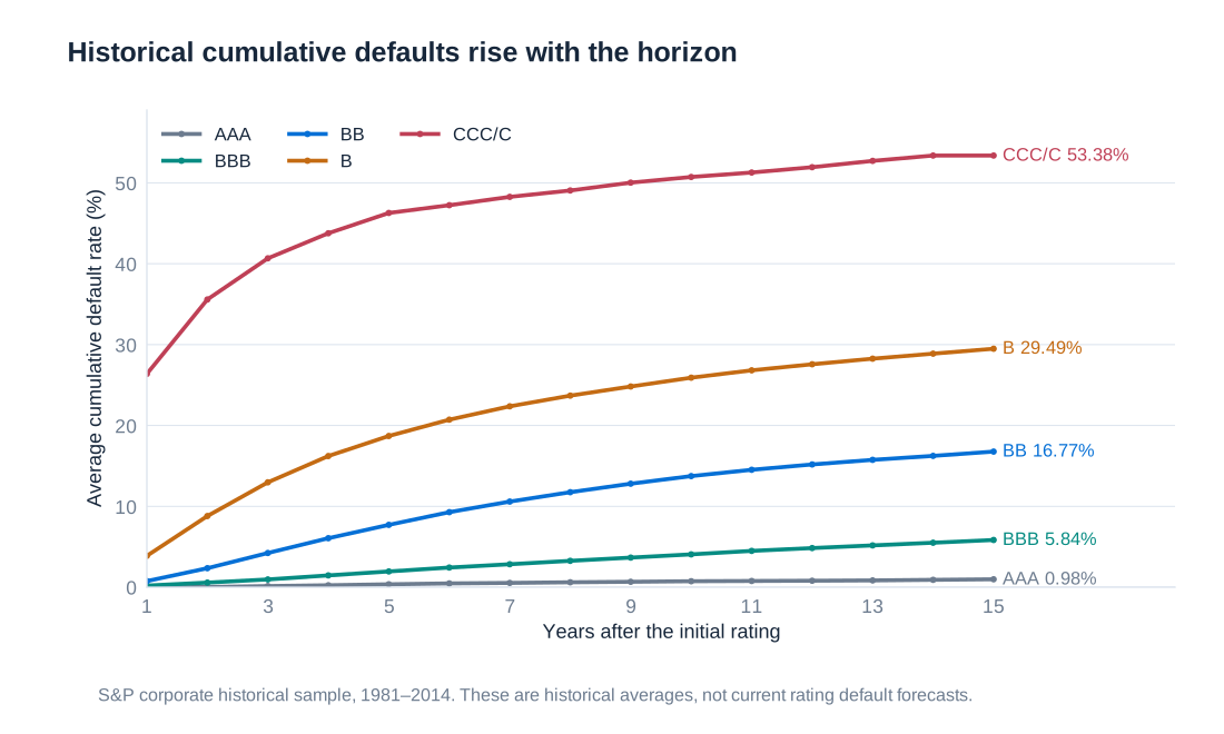
For example, the historical BBB rate is 0.20% at one year and 1.95% at five years, whereas the corresponding B rates are 3.88% and 18.70%. Cumulative default probability rises with the horizon, but annual increments need not be constant. An initially strong borrower has time to deteriorate; an initially weak cohort also changes composition as vulnerable firms default and survivors remain. Consequently, multiplying a one-year rate by the number of years is not generally a sound method of estimating a multi-year PD.
Let denote cumulative default probability, with default time and . The unconditional probability of default during year is . The conditional probability, given survival to the beginning of that year, is
For the BBB observations, the second-year unconditional increment is . The corresponding conditional probability is . These quantities are close for a low-risk cohort but differ materially when cumulative default rates become large. Under a constant annual conditional probability , survival through years is and cumulative PD is .
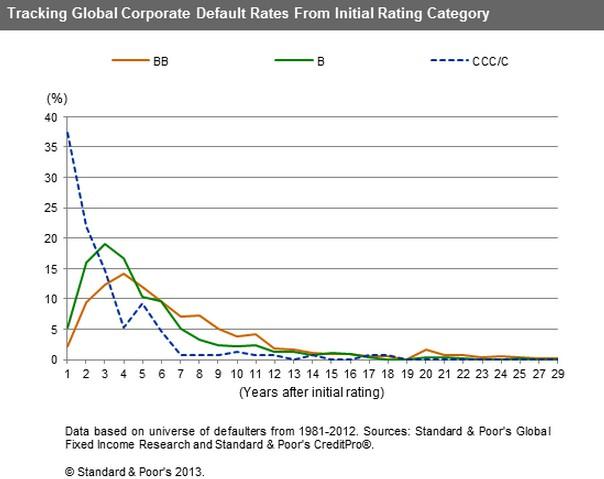
The historical timing graphic below has a different denominator: it tracks the timing of defaults among firms that ultimately defaulted in its 1981–2012 sample, grouped by initial rating. It illustrates how quickly eventual defaulters reached default. Its percentages must not be read as unconditional annual PDs for all firms initially assigned a rating or used interchangeably with the cumulative-rate table.
Internal scores, financial ratios and classification
An internal rating starts with quantitative and qualitative information about an obligor. A basic score may then be changed by warning signals, exceptional circumstances, support from a parent or guarantor, and a documented override. The resulting obligor grade should be distinguished from an assessment of a particular facility: collateral and seniority can materially change LGD without improving the borrower's ability to avoid default. A score is ordinal if it only ranks borrowers; it becomes a metric measure of risk only after calibration to a probability or expected-loss quantity.
A linear score has the form , where are borrower characteristics and are fitted coefficients. Profitability and leverage often move creditworthiness in opposite directions, but the score's sign convention must be specified. If higher means stronger credit, a profitability coefficient may be positive and a leverage coefficient negative. Combining these dimensions creates a boundary between classifications; it does not establish that the chosen ratios alone cause future default.
The following historical illustration uses an Altman-style modified score:
where is working capital divided by total assets, retained earnings divided by total assets, EBIT divided by total assets, and market value of equity divided by book liabilities. This is the particular specification used in the illustration, not a universal Altman formula: published Z-score variants differ in coefficients, equity definitions and the population for which they were developed. Mixing one variant's inputs with another variant's thresholds invalidates the interpretation.
| Input or result | BMW | Daimler |
|---|---|---|
| Working capital | −0.25 | 3.18 |
| Retained earnings | 20.42 | 19.36 |
| EBIT | −0.22 | 3.48 |
| Market value of equity | 19.28 | 25.46 |
| Sales (not used in this formula) | 51.42 | 87.49 |
| Total assets | 101.86 | 127.28 |
| Book liabilities | 79.70 | 96.67 |
| Calculated score Z | 4.13 | 4.37 |
| Illustrative score-mapped grade | B | B+ |
The displayed inputs produce for BMW and for Daimler. The B and B+ labels belong to this illustration's score mapping, not to a verified claim about either company's actual agency rating in 2008. The source's monetary scale is ambiguous, so the table preserves the common-scale inputs and explicitly treats them as ratio-building data rather than audited euro amounts. Sales are shown for completeness but do not enter this particular four-ratio formula. Rescaling all monetary inputs by the same factor leaves every ratio and the score unchanged.
Any classification cutoff creates two kinds of error: a borrower later defaults after being classified as acceptable, or a borrower that would repay is classified as unacceptable. These are sometimes called Type I and Type II errors, but naming conventions differ. Stating the event explicitly is safer. Lowering approval standards can increase lending and interest income while admitting more eventual defaults. Tightening standards reduces that exposure but rejects some profitable good borrowers. The appropriate cutoff depends on losses, margins, operating costs and constraints, not on classification accuracy alone.
Logistic models and retail information
A logistic model maps a linear index to a number between zero and one:
The log-odds satisfy . A positive coefficient raises PD when the associated variable increases, holding the others fixed; its effect on probability is nonlinear and depends on the initial PD. As a purely mathematical illustration, crosses 50% at . Here is a dimensionless illustrative stress index. These coefficients are not presented as an estimated or validated credit model, and they must not be used to approve a loan.
Retail credit assessment may use income and expenditure information supplied to the lender, assets and existing liabilities, employment stability, contractual loan features and observed payment behaviour. Account conduct can reveal persistent overdrafts, irregular inflows or missed payments. Credit registries can add information about obligations with other institutions and adverse payment events. No single variable substitutes for a documented assessment of repayment capacity, and a registry score is not the same thing as the lender's affordability calculation.
Historical lists of potential model inputs include demographic characteristics, residential location and behavioural proxies. Such availability does not make an attribute appropriate to use. Data relevance, accuracy, lawful processing, discriminatory effects and the possibility that apparently neutral variables proxy protected characteristics require separate assessment. Information collected for credit assessment also needs a defined retention policy and a way to correct errors; a historical example of a retention period is not a rule applying to every record today.
SCHUFA provides a useful example of a German credit-information system. Its records can include identifying information, credit and account relationships, inquiries and payment disruptions. Its new score introduced in March 2026 uses 12 criteria and a scale from 100 to 999. These criteria concern payment disruptions; the age of the oldest bank contract and oldest credit card; address tenure; the age of the youngest revolving facility; recent banking and non-banking inquiries or contracts; recent instalment loans and their longest remaining maturity; credit status; mortgages; and identity checks. SCHUFA states that it does not know a person's income, wealth, marital status or religion.
Current description: SCHUFA's twelve score criteria and information not held by SCHUFA. The score's introduction date and criteria replace older, inconsistent descriptions.
A December 2025 newspaper example concerning a credit-card provider change illustrates why consumers may question changes in a registry score even when their income has not changed. The case concerns a historical scoring environment and does not establish the effects of every card switch under the later model. The general analytical point is that a statistical score responds to the information and design of that model, whereas actual repayment capacity also depends on circumstances outside it.

Calibration, discrimination and validation
A model can rank borrowers well while producing inaccurate probabilities, or produce a reasonable portfolio average while ranking individuals poorly. Calibration asks whether predicted PDs agree with observed default frequencies over the relevant horizon. Discrimination asks whether eventual defaulters receive worse scores than survivors. Stability asks whether these properties persist across time, industries and borrower populations. Validation must examine all three rather than treating a single goodness-of-fit statistic as sufficient.
For corporate portfolios, quantitative financial ratios are supplemented by forecasts, management quality, competitive position and industry conditions. An accounting-based rating need not react immediately to market spreads; a market-implied model will respond faster but also incorporates risk premia and liquidity. A through-the-cycle system and a point-in-time system can legitimately behave differently. Calibration requires a default definition, a reference population, a horizon and representative data, including downturns where available. Regulatory IRB standards impose data-history and conservatism requirements. For corporate PD estimation, the historical observation period must cover at least five years; longer relevant available histories should be used. Five years of history are not the same as five borrower observations, and meeting a minimum period alone does not make a model reliable.
Data-history reference: Basel CRE36 minimum requirements for IRB models.
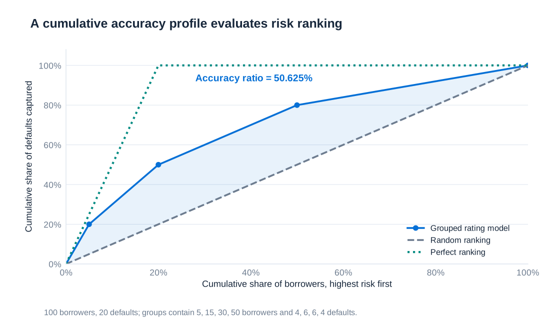
Consider two illustrative classifications of the same-sized portfolio of 100 loans with 20 eventual defaults. Classes are ordered from highest to lowest risk. In example A, default rates are 60%, 40%, 20% and 8%; example B changes the first two class sizes and default counts. Keeping the examples separate matters because their accuracy ratios are similar but not identical.
| Risk class | A: loans | A: defaults | A: default rate | B: loans | B: defaults | B: default rate |
|---|---|---|---|---|---|---|
| 1 (highest risk) | 10 | 6 | 60% | 5 | 4 | 80% |
| 2 | 10 | 4 | 40% | 15 | 6 | 40% |
| 3 | 30 | 6 | 20% | 30 | 6 | 20% |
| 4 (lowest risk) | 50 | 4 | 8% | 50 | 4 | 8% |
| Total | 100 | 20 | 20% | 100 | 20 | 20% |
A cumulative accuracy profile, or CAP, plots the proportion of all eventual defaults captured against the proportion of borrowers selected, starting with the riskiest scores. Random ranking follows the diagonal. Perfect ranking places all 20 defaults first, reaches 100% of defaults after 20% of borrowers, and is flat thereafter. The accuracy ratio is the area between the model curve and the random diagonal divided by the corresponding area for perfect ranking.
For example B, the CAP points are , , , and . Joining these points linearly, the area under the curve is 0.7025. The random area is 0.5 and the perfect area is 0.9, so
Example A gives an area of 0.7000 and an accuracy ratio of 50%. These figures measure ranking power for the constructed samples; they do not mean that the model predicts each default with 50% accuracy. A good validation also checks calibration by grade, uncertainty from small samples, overrides, data quality and out-of-sample performance. Perfect retrospective ranking can reflect overfitting rather than usable forecasting ability.
Credit deterioration, accounting losses and capital pressure
The financial crisis exposed weaknesses in securitisation ratings, internal-model incentives, counterparty assessment and reliance on apparently safe sovereign assets. Complex structures could concentrate systematic exposures while appearing diversified. Institutions could also postpone recognition of weak lending through repeated refinancing or restructuring that failed to restore sustainable repayment capacity. A new contractual maturity does not by itself cure an economic credit problem.
Policy responses included changes to trading-book and securitisation capital, stronger treatment of non-performing exposures, limits on internal-model variability, stress testing, and collateral or central-clearing requirements for eligible derivatives. These address different channels: a capital rule increases resilience to loss, a stress test studies adverse scenarios, and collateral reduces unsecured counterparty exposure. None makes underlying borrower defaults impossible. The historical term Basel 2.5 refers to an earlier set of trading-book reforms, whereas CRR3 implements later revisions in the EU.
Fair-value measurement also needs care. Level 1 uses quoted prices in active markets for identical assets or liabilities; Level 2 uses other observable inputs; Level 3 uses significant unobservable inputs. The hierarchy concerns valuation inputs, not a permanent classification of entire security types. A valuation adjustment may reflect counterparty credit risk (CVA), own credit risk (DVA), funding effects (FVA) or liquidity assumptions sometimes described as LVA. These labels do not justify mechanically adding overlapping discounts: the valuation method and applicable accounting rules must avoid double counting.
For the input hierarchy, see IFRS 13 Fair Value Measurement.
A broad credit shock can hit a bank through several routes simultaneously. New defaults and revised recoveries increase credit losses; deteriorating performing exposures can require greater expected-loss allowances; traded credit assets can fall in fair value; and higher PDs, LGDs or weaker ratings can increase RWA. Earnings and capital may therefore fall while the capital requirement rises. Attempts by many banks to reduce lending at the same time can amplify a downturn through a credit crunch.
A historical first-quarter 2020 Credit Suisse example makes these distinctions concrete. The original figures are in CHF millions, not euros, and the allowance treatment refers to US GAAP CECL rather than IFRS 9. Credit-loss provisions are not limited to losses on loans that have already defaulted. The following bridge keeps allowance movements and fair-value marks separate before reproducing the broader reported reserve-build measure.
| Component | Amount | Interpretation |
|---|---|---|
| Credit-loss provisions | 568 | Income-statement charge; includes expected losses |
| Net write-offs and other allowance movements | −55 | Other changes in the allowance |
| CECL adoption effect | 72 | Transition effect included in the allowance increase |
| Increase in credit-loss allowance | 585 | 568 − 55 + 72 |
| Leveraged-finance fair-value marks | 284 | Separate mark-to-market component |
| Asia-Pacific financing fair-value marks | 160 | Separate mark-to-market component |
| Total fair-value marks | 444 | 284 + 160 |
| Total reported reserve build | 1,029 | 585 + 444 |
| Of which: CECL-related component | 376 | 72 adoption + 304 additional build; already included above |
| Other component of reported reserve build | 653 | 1,029 − 376; not an additional charge |
The CHF 376 million CECL-related component consists of the CHF 72 million adoption effect and CHF 304 million of additional allowance build; it is part of the total, not a further amount to add to CHF 1,029 million. The remaining CHF 653 million completes that presentation. This example shows why a headline reserve-build number must be reconciled to its components before being interpreted as realised default losses or as a single accounting provision charge.
Portfolio loss, dependence and economic capital
A portfolio model combines individual exposure characteristics with the way defaults, migrations and recoveries co-move. Independent small exposures diversify more effectively than a few large exposures or many borrowers linked to the same sector, region or economic factor. Expected loss adds across borrowers regardless of dependence, but the tail of the total-loss distribution can change dramatically. A portfolio can therefore have the same EL as another and need much more capital to absorb adverse outcomes.
Write borrower loss as , where equals one after default and zero otherwise. Total loss is . Its variance includes both individual variances and pairwise covariance terms:
Independence removes the covariance terms, but it is a strong assumption. A recession can simultaneously increase default probabilities, reduce collateral prices and lengthen recovery procedures. This creates adverse dependence between default rates and LGDs, so a constant recovery assumption can understate severe losses. Shared counterparties, supply chains and funding sources can add concentration beyond broad sector labels.
In a one-factor Gaussian model, a latent asset return is , where the systematic factor and idiosyncratic shocks are independent standard normal variables. Borrower defaults if . Conditional on , its PD is . The parameter is an asset-factor correlation, not the default-indicator correlation itself.
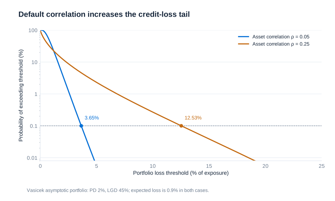
For an infinitely granular homogeneous portfolio with constant LGD, the model's loss-rate quantile is
With PD 2%, LGD 45% and a 99.9% confidence level, increasing from 0.05 to 0.25 raises the quantile from approximately 3.6465% to 12.5323% of total exposure, although EL remains 0.9%. This is a different, asymptotic model from the earlier finite portfolio of 100 independent loans. The graph compares exceedance probabilities on a logarithmic vertical scale: a 0.1% tail probability marks the 99.9% quantile.
Monte Carlo simulation implements more elaborate versions by repeatedly drawing common factors and borrower outcomes, applying exposures and recoveries, and collecting total losses or changes in value. The average simulated loss estimates EL; a selected quantile estimates VaR; their difference measures quantile-based economic capital under the stated convention. A 99.98% confidence level is one possible internal choice, not a universal requirement. A higher confidence level also makes tail estimation more demanding, especially when extreme losses are rare.
CreditMetrics and migration risk
A default-only model ignores losses from worsening credit quality before default. CreditMetrics-style models instead allow each borrower to migrate among rating states over a horizon. Each non-default state receives a horizon value obtained by discounting the remaining cash flows using rates appropriate to that state. The default state receives a recovery value. The resulting distribution includes gains from upgrades, losses from downgrades and losses from default.
A transition matrix states the probabilities of moving from each initial rating to each ending rating. The historical matrix below is an adjusted example from the CreditMetrics technical document, based on S&P transition information and adjusted to match long-term probabilities. It is not a current matrix or an unadjusted Moody's estimate. Values are percentages; the absorbing default row is added explicitly as 100%, not 1%. Small deviations of a row sum from 100% reflect the displayed rounding.
| Initial rating | AAA | AA | A | BBB | BB | B | CCC | Default |
|---|---|---|---|---|---|---|---|---|
| AAA | 87.74 | 10.93 | 0.45 | 0.63 | 0.12 | 0.10 | 0.02 | 0.02 |
| AA | 0.84 | 88.23 | 7.47 | 2.16 | 1.11 | 0.13 | 0.05 | 0.02 |
| A | 0.27 | 1.59 | 89.05 | 7.40 | 1.48 | 0.13 | 0.06 | 0.03 |
| BBB | 1.84 | 1.89 | 5.00 | 84.21 | 6.51 | 0.32 | 0.16 | 0.07 |
| BB | 0.08 | 2.91 | 3.29 | 5.53 | 74.68 | 8.05 | 4.14 | 1.32 |
| B | 0.21 | 0.36 | 9.25 | 8.29 | 2.31 | 63.89 | 10.13 | 5.58 |
| CCC | 0.06 | 0.25 | 1.85 | 2.06 | 12.34 | 24.86 | 39.97 | 18.60 |
| Default | 0.00 | 0.00 | 0.00 | 0.00 | 0.00 | 0.00 | 0.00 | 100.00 |
Each row conditions on the initial rating, so reading the table by columns answers a different question. For example, the BBB row assigns 84.21% to remaining BBB and 0.07% to default over the model horizon. The table cannot alone predict the starting composition of a portfolio or the fraction of defaults originating in BBB. When it is used numerically, minor rounding discrepancies should be handled transparently, for example by normalising the displayed row within its rounding tolerance.
If the transition mechanism is assumed stationary and Markovian, a multi-period transition matrix is a power of the one-period matrix: . This assumption says that the current rating contains the relevant migration information and the probabilities remain stable. Rating history, the business cycle and changing market conditions can violate it. Multiplying matrices is therefore a modelling operation, not a factual statement that historical transitions will repeat.
Portfolio implementation needs dependence between migrations as well as individual transition probabilities. CreditMetrics uses a latent-variable framework in which rating thresholds and asset-return correlations generate joint states; equity-return information may be used as a proxy when suitable. Each simulated joint outcome is then revalued. Recovery assumptions, concentration and the sensitivity of state values to interest rates and credit spreads can all affect the tail. Model comparison should keep the horizon, valuation basis and confidence level consistent.
Historical matrix and methodology: CreditMetrics Technical Document, Table 6.11. The example is preserved as a historical model illustration.
Managing the exposure and its residual risks
Credit-risk management begins before a loan is made: underwriting, exposure limits, pricing, covenant design and sector diversification determine the initial risk. Monitoring then tracks financial deterioration, missed payments and other warning signals. Collateral can lower loss severity if it is legally enforceable and retains value in the default scenario. A guarantee transfers exposure to the guarantor and must be assessed in light of that party's own capacity and possible correlation with the borrower.
Contractual tools can include material-adverse-change clauses, review or cancellation rights for uncommitted facilities, and shorter refinancing periods. Their practical effect depends on the agreement and applicable law. They may limit future lending but do not automatically recover money already advanced. A withdrawal of liquidity can also worsen the borrower's position, which makes early monitoring and orderly restructuring more useful than a purely mechanical response to a score.
Netting reduces exposure only when the relevant arrangements are legally effective and cover the obligations in question. Derivative protection introduces counterparty risk; a securitisation can leave retained tranches, servicing obligations or contingent liquidity facilities. The historical IKB/Rhineland experience illustrates why an apparently separate vehicle can return risk to a sponsoring bank through support commitments or funding stress. An off-balance-sheet label is therefore not enough to establish economic risk transfer.
CDS and asset-backed structures provide additional tools for altering the distribution of credit exposure. Their value lies in the precise contractual transfer they achieve, not in removing credit risk from the financial system. The next chapter follows their cash flows, identifies who bears each loss, and separates credit protection from funding, liquidity and counterparty effects.