
3. Commodity Price Risk and Minimum-Variance Hedging
Commodity risk arises because the prices, quantities and delivery conditions of physical inputs and outputs change. An airline purchases fuel, an oil producer sells petroleum, and a manufacturer may be exposed on both sides through energy costs and product prices. Their exposure is the effect on the whole business, not simply the movement of one quoted commodity price. A derivative can offset that exposure, but its effectiveness depends on matching the commodity, quantity, maturity and cash-flow timing. Price protection can therefore coexist with basis risk, counterparty risk or a serious demand for cash.
Trading rewards, operating exposures and the purpose of a hedge
In December 2023, reporting on Goldman Sachs trader Ed Emerson put his three-year compensation near USD 100 million, illustrating potential commodity-trading rewards. Such examples must be distinguished from the objective of a corporate hedging programme. A trader may earn money by supplying liquidity, intermediating client transactions or deliberately accepting market exposure. An operating company normally hedges to stabilise an input cost, selling price, cash flow or balance-sheet value. The fact that a derivative loses money does not establish that the hedge failed: that loss may accompany an economically valuable gain in the underlying business.
A producer expecting to sell a known quantity is adversely exposed to falling prices; a consumer expecting to purchase it is adversely exposed to rising prices. The producer generally needs a short price hedge and the consumer a long price hedge. This directional rule applies to the specified exposure, not automatically to the company's name or industry. An oil distributor that has promised fixed-price deliveries but has not yet acquired the oil is exposed to rising acquisition costs, even though it will ultimately be selling the commodity to customers.
The risk-management objective should specify the quantity, delivery location, quality, currency and dates of the exposure, together with the loss measure and horizon. Hedging a price per barrel does not by itself hedge an uncertain number of barrels. Likewise, a crude-oil contract does not exactly hedge jet fuel, which includes refining and product-specific market effects. These distinctions explain why an apparently simple one-for-one hedge can leave substantial risk.
Forward contracts, futures and settlement obligations
A long forward commits its holder to buy a specified underlying at a delivery price agreed today; a short forward commits its holder to sell. Let be the agreement date, the delivery date, the spot price at delivery and the agreed delivery price per unit. Ignoring costs and default, the terminal economic payoffs are
For physical delivery, the long party pays and receives an asset worth . Cash settlement pays the economically equivalent difference when the contract specifies it. These are linear payoffs: a one-unit increase in the terminal price raises the long payoff by one unit and lowers the short payoff by one unit. For units of the underlying, multiply the payoff by .
A forward agreed at the current fair delivery price normally has zero initial market value. Zero initial value does not mean zero risk, zero future liability or unlimited access to funding. A contract agreed away from the fair price has a nonzero value, and collateral arrangements can require cash before maturity. Bilateral forwards also expose each party to the possibility that an in-the-money counterparty fails to perform.
Exchange-traded futures are standardised contracts supported by a clearing and margin system. Initial margin is a performance deposit; variation margin transfers gains and losses as the contract is marked to market. The clearing structure substantially reduces bilateral counterparty exposure, but it does not eliminate every clearing-member, operational, liquidity or extreme default risk. Futures may end in physical delivery or cash settlement. Closing a position before expiry requires an offsetting trade in the relevant contract, not merely a decision to stop recognising its value.
| Feature | Forward | Futures |
|---|---|---|
| Contract terms | Usually negotiated bilaterally | Standardised by the trading venue |
| Initial value and funding | Normally zero fair value at inception; collateral may be required | Initial margin is posted |
| Settlement during the contract | Depends on collateral and contractual arrangements | Variation margin settles marked-to-market gains and losses |
| Principal risk-management consequence | Counterparty exposure and contractual collateral terms matter | Immediate cash requirements can arise despite an economically offsetting exposure |
How a matched forward fixes a purchase cost
Suppose a consumer must buy one unit at and enters a long forward with currency units. The physical purchase costs , while the forward produces . The net cost after the hedge is therefore
If the price rises to 100, the physical cost is 100 and the derivative gain is 20. If the price falls to 60, the physical cost is 60 and the derivative loss is 20. Both cases give a net cost of 80. Evaluating only the derivative in the second case would miss the offsetting saving on the actual purchase. A producer selling one unit would instead combine sale revenue with a short forward, giving .
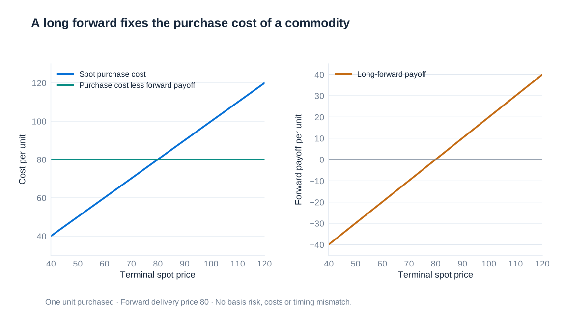
The cancellation requires the purchase and hedge to concern the same underlying, quantity and date and assumes performance by the counterparties. A similar example is a payment of USD 1 million due in three months hedged by a three-month forward that supplies exactly that dollar amount. The exchange-rate exposure of that payment can be removed, although funding, credit and operational risks remain. In a commodity business these matching conditions are often harder to achieve.
Cash-and-carry pricing and its assumptions
For a freely tradable asset that pays no income and has no storage costs, spot and forward prices are linked by financing. Let be the current spot price, the fair forward delivery price, a continuously compounded financing rate per year and the remaining time in years. Buying the asset today and financing it until delivery costs at . Equivalently, a fair long forward plus an investment that grows to the delivery payment produces the same terminal asset. No arbitrage therefore requires
If a forward price were above this financing-adjusted spot price, an investor able to borrow, purchase and store the asset could sell it forward and lock in a difference. The reverse trade requires the ability to short or otherwise obtain the underlying. Transaction costs, credit limits and restrictions on short selling can therefore create bounds rather than an exact relationship in practice.
For example, with a spot price of EUR 80, a continuously compounded annual financing rate of 5% and six months to delivery, the no-income, no-storage calculation is , or approximately EUR 82.03. The difference from the spot price is financing compensation, not automatically a forecast that the future spot price will rise by that amount. Forward prices and expected future spot prices need not coincide because risk premia and other economic forces can matter.
Valuing an existing forward before maturity
The delivery price of an existing contract remains fixed while the fair delivery price for new contracts changes. Suppose an earlier long forward has delivery price . At a later date , an opposite short forward with the same underlying and maturity can be entered at the new fair price . At maturity, the physical obligations offset and the combined payoff is . Under the simple deterministic-rate assumptions, the current value of the original long forward is
If the original delivery price was USD 10 and the new forward price is USD 11, the offset locks in USD 1 per unit at maturity. Its value today is the discounted dollar, not automatically exactly USD 1. The offset removes the price exposure but does not necessarily terminate both contracts or remove their counterparty and collateral obligations. Close-out and netting arrangements determine the contractual result.
Changes in forward prices are consequently a useful approximation to changes in forward value when discounting effects over the interval are small. Futures variation margin, by contrast, is paid or received during the contract's life. Under deterministic interest rates and otherwise identical terms, standard forward and futures prices coincide; with stochastic rates, the relationship between settlement cash flows and rates can produce a difference. The timing of gains and losses is economically relevant even when terminal price exposure appears similar.
Storage costs, convenience yield and the forward curve
Physical inventory can be costly to finance, insure and store, but possessing it can also provide an operating benefit. A refinery with available crude can keep producing during a supply disruption; a firm without inventory may miss a sale or interrupt production. Convenience yield represents this noncash benefit of holding the physical commodity. With proportional storage costs and convenience yield , both expressed as annual continuous rates, a common cost-of-carry representation is
Financing and storage tend to raise the forward price relative to spot, while convenience yield tends to lower it. Contango commonly describes a forward price above spot or an upward-sloping curve across maturities; backwardation describes the opposite configuration. These related usages should be stated clearly. A high convenience yield can support backwardation despite positive financing and storage costs. As a deliverable contract reaches maturity, its price converges to the corresponding spot delivery value under the contract's delivery and settlement rules.
The formula is most informative when the underlying inventory and arbitrage assumptions are credible. Electricity is difficult to store economically at large scale, agricultural goods have seasonality and deterioration, and livestock involve biological production and maintenance. Location, quality and transport constraints further segment markets. Spot and deferred prices can consequently respond differently to the same news. That does not mean that the markets are literally unrelated; it means that a simple immediate storage trade may not enforce a tight price link.
For positive observed prices, an implied convenience yield can always be calculated as . If this unknown is chosen solely to fit the observed forward price, however, the equation becomes a decomposition rather than an independent prediction. A collapse in current oil demand can depress nearby prices more than deferred prices as inventories accumulate and storage becomes scarce. The change in curve shape is then as important to a rolling hedge as the change in the overall price level.
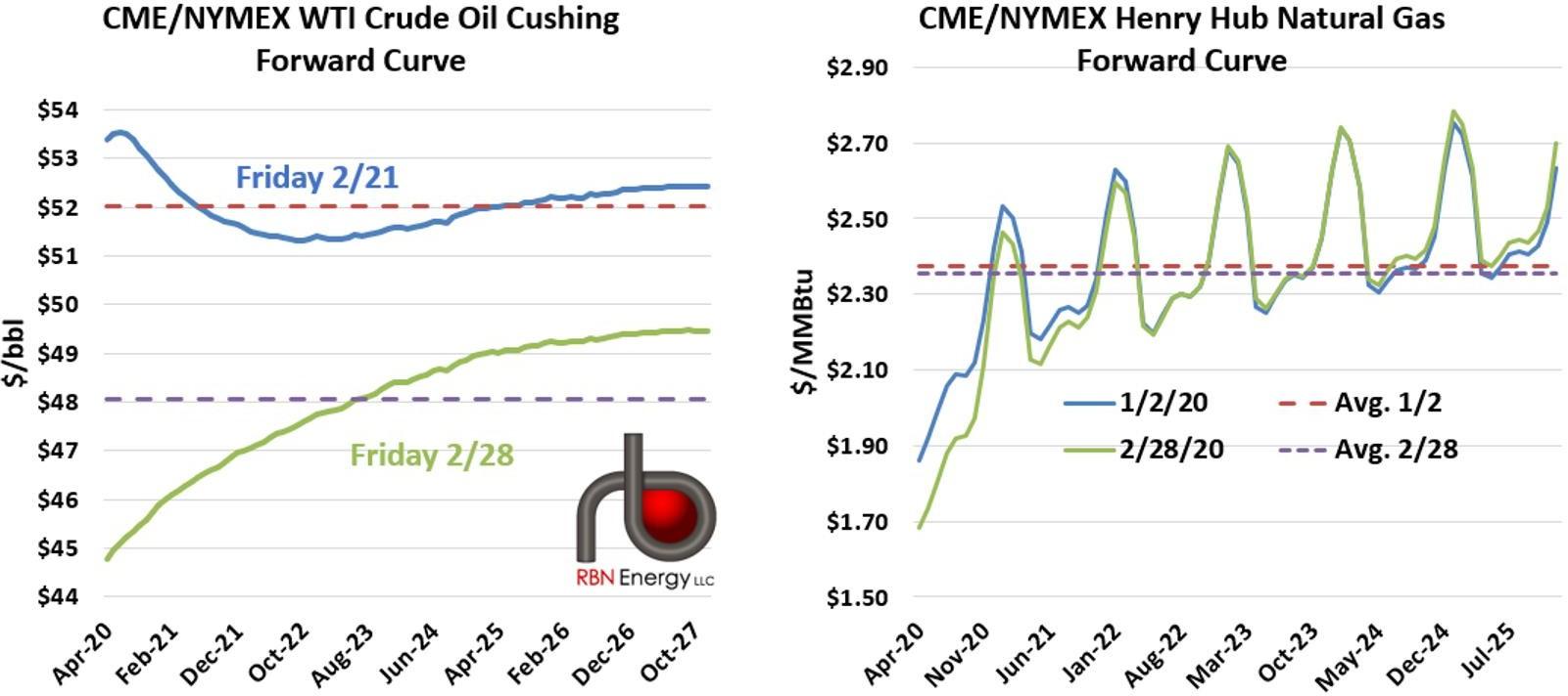
The February 2020 oil-curve comparison illustrates this distinction: nearby and deferred WTI prices both moved, but the size of the decline depended on the delivery month. Comparing entire curves reveals changes in term structure that a single spot-price observation would conceal. These are dated market observations, not a prediction of how every future demand shock must affect the curve.
Basis risk and the minimum-variance hedge
A cross-hedge uses an instrument that is related to, but not identical with, the exposure. Hedging jet fuel using crude-oil futures is an example: the jet-fuel bill and crude futures usually respond to common energy factors but also have separate influences. A hedge can also have maturity basis risk when short-dated contracts are rolled against a long-dated exposure. The relevant relationship is between changes over the actual risk horizon, not simply between long-run price levels.
Let be the unhedged change in the value of the business exposure, in currency, and let be the profit on one long futures contract over the same interval, also in currency. Let be the signed number of contracts: positive means long and negative means short. The hedged value change and its variance are
where , and . Differentiating with respect to gives . If the hedge contract has positive variance, the unique minimum is
where is the correlation of exposure changes and long-contract profits. The minus sign makes the position offset the exposure. A long inventory position generally has positive covariance with a long commodity future, requiring a short hedge. A future purchase cost enters business value with a negative sign; its adverse exposure generally calls for a long hedge. Defining the exposure as a cost instead of value is possible, but then the hedge payoff must be subtracted rather than added.
Contract size, regression estimation and remaining risk
If the exposure is units of inventory at spot price and each futures contract covers units with futures price , then and . The optimal signed number is
This distinguishes a dimensionless price hedge ratio from an actual contract count. For an illustrative inventory of 10,000 units, a contract size of 100 units, correlation 0.8 and a spot-change standard deviation 1.25 times the futures-change standard deviation, the price hedge ratio is . The optimal position is therefore contracts. Rounding, transaction costs and trading limits can make the feasible position differ from the continuous optimum.
Regressing on an intercept and estimates the slope . This is the positive hedge-size coefficient when covariance is positive; the signed inventory hedge is its negative after quantity conversion. The intercept captures an average change and does not itself reduce variance. Estimates should use observations relevant to the intended horizon and be checked for changes in market conditions rather than treated as permanent constants.
Substituting the optimal hedge into the variance expression gives
With a single regressor and an intercept, the regression's equals and measures the fraction of in-sample variance eliminated. Correlation 0.5 removes only 25% of variance; zero correlation offers no variance reduction. Perfect positive or negative correlation permits zero residual variance in this ideal linear model if either hedge direction is available. At correlation 0.7, 51% of the original variance remains and residual standard deviation is approximately 71.41% of its original level.
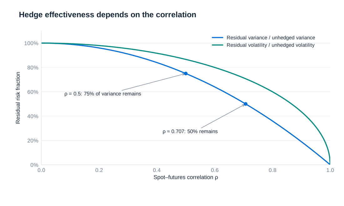
If , as in an illustrative single-stock hedge using index futures, half the variance remains but the remaining standard deviation is , or about 70.7%, not 50%. This distinction is also essential when assessing commodity hedges. Variance efficiency measures a particular price-risk objective; it does not measure the ability to finance margin calls or guarantee that an estimated relationship will hold during a crisis.
When the underlying business disappears: Lufthansa in 2020
A forecast purchase is not the same as an unconditional obligation. The pandemic-related collapse in aviation activity reduced Lufthansa's fuel and currency needs, leaving some previously designated hedges without the forecast transactions they had been intended to offset. Falling fuel prices could then generate derivative losses without a matching saving on fuel that was no longer purchased. An excessive hedge became a separate open exposure.
Lufthansa's 2020 reporting identified EUR 758 million of realised fuel-hedge expenses and EUR 28 million of realised foreign-currency hedge earnings on expired stand-alone derivatives, a net result of EUR −730 million. These figures concern that specified category of derivatives, not the airline's total annual loss or its entire hedging result. The lesson is that volume forecasts, contractual commitments and hedge quantities must be reviewed together. A decision about whether to retain, reduce or close an overhedge also needs the resulting market-value and cash consequences.
Primary source: Lufthansa Annual Report 2020, page 213.
Metallgesellschaft: long-term promises and short-term cash demands
The Frankfurt-based industrial group Metallgesellschaft's oil-related crisis developed in 1993–94 and led to an emergency recapitalisation of the German parent company, rather than a simple completed bankruptcy. The core economic problem involved long-term fixed-price petroleum delivery contracts and large positions in short-term derivatives. The crisis combined price exposure, maturity mismatch, funding requirements and weaknesses in oversight; it cannot be understood by looking only at the final payoff of one futures contract.
A simplified delivery commitment makes the direction clear. If a distributor promises one barrel every month for ten years at a fixed selling price, it has committed to 120 future barrels. Higher purchase prices would reduce its delivery margin. Long oil futures can therefore offset the adverse price direction. But holding near-term futures for all 120 barrels concentrates exposure at the front of the curve, whereas the physical deliveries occur over 120 separate months. Short-term contracts must be rolled and adjusted as deliveries occur.
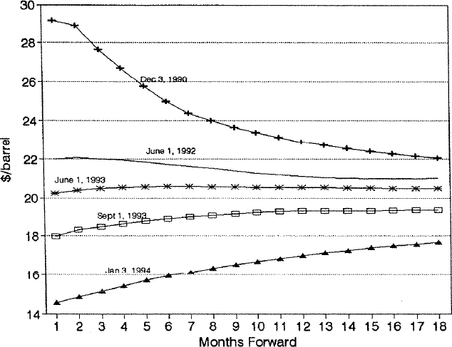
When oil prices fell and the curve moved toward contango, long near-term futures generated losses that demanded immediate cash. Fixed-price customer sales could become more valuable because oil could eventually be purchased more cheaply, but those benefits were spread across future deliveries and were not equivalent to cash available for today's margin call. Different maturities also moved by different amounts, so an economically offsetting direction did not imply an equal offset in present value.
Rolling introduces another mismatch. A long position is closed in the expiring contract and reopened further out. In contango, the new contract may be more expensive than the old one, changing the economics of maintaining exposure. This difference is not necessarily an immediate payment of the whole futures notional: futures are margined contracts. Nevertheless, the evolution of prices, repeated settlements and financing of collateral determine the realised cash-flow path. A hedge that requires funding the company cannot obtain may be impossible to maintain.
Historical analysis: Frankel and Palmer, Federal Reserve International Finance Discussion Paper 560 (1996).
Evaluating hedge size and the complete risk budget
Historical regression estimates associated with the Metallgesellschaft debate illustrate why matching total barrels one-for-one need not minimise variance. The table relates changes in longer-dated futures prices to changes in the nearest one-month futures price over 1990–1992. The slope estimates below one indicate that a unit change in the near-term price was associated with a smaller change in the longer-dated contract; the relationship also varied by product and maturity.
| Contract maturity | Heating oil: slope | Heating oil: R² | Gasoline: slope | Gasoline: R² |
|---|---|---|---|---|
| Two months | 0.735 | 0.84 | 0.740 | 0.80 |
| Three months | 0.625 | 0.79 | 0.650 | 0.75 |
| Six months | 0.513 | 0.80 | 0.562 | 0.76 |
| Nine months | 0.492 | 0.79 | 0.520 | 0.72 |
For example, the six-month heating-oil slope of 0.513 implies a smaller offsetting near-term price exposure than a one-for-one position, under that regression's units and assumptions. Its of 0.80 implies 20% residual variance and about 44.72% residual standard deviation in the fitted single-factor model. These short-maturity historical estimates do not by themselves determine a ten-year delivery programme's optimal hedge. They demonstrate the need to estimate the relevant price relationship rather than assume equal sensitivities.
A hedge also needs clear responsibility for monitoring positions, approving exceptions and arranging collateral before a stressed market closes access to finance. A complete hedge policy combines exposure measurement, a defensible contract size, stress tests of curve changes and volume disruption, and a funding plan for adverse margin paths. Long-term delivery optionality and customer credit risk require separate analysis. Minimum variance is one useful objective, but management may instead need to protect minimum cash balances or avoid a severe funding shortfall. Those objectives can justify a hedge smaller than the unconstrained variance optimum, a different maturity structure or a different instrument.