
4. Interest Rate Risk, Duration and Banking-Book Exposure
Interest rates influence both the present value of promised cash flows and the income earned when money is reinvested or funding is renewed. A fixed-rate bond can lose market value when yields rise even though its contractual payments have not changed. A saver rolling short-term deposits can instead be harmed by falling future rates, while a bank faces the combined repricing of assets, liabilities and derivatives. Interest-rate risk management therefore begins by specifying the cash flows, the valuation convention and the horizon over which risk is being assessed.
Market-value risk and reinvestment risk
Market-value risk is the possibility that changing discount rates reduce the current value of an asset or increase the current value of a liability. For a conventional fixed-rate bond, higher required yields reduce present value because the same future payments are discounted more heavily. Reinvestment risk concerns the uncertain rates available when coupons, principal repayments or other cash receipts must be invested again. These risks can move in opposite directions: a fall in rates raises the current price of a fixed-rate bond but reduces the income available on future reinvestment.
Suppose an investor repeatedly purchases one-year instruments over a 30-year saving horizon. Ignoring costs and default, terminal wealth from an initial amount is , where is the one-year rate available for year . The first rate may be known, but the later rates are not. Short contractual maturity therefore does not eliminate uncertainty about long-horizon wealth. A pension institution must relate the timing and size of its assets to the timing and size of its benefit obligations.
The relevant objective might be tomorrow's liquidation value, next year's net interest income or the funding of a payment decades away. The same security can look relatively safe under one objective and risky under another. Inflation, credit risk and liquidity can add further uncertainty even when a contractual nominal payment is fixed. A duration calculation isolates a specified interest-rate sensitivity; it is not a complete statement about every risk of holding a bond.
Zero-coupon bond valuation and yield to maturity
A default-free zero-coupon bond makes one payment at maturity. Let denote its face value, its remaining maturity in years and its effective annual yield to maturity. With annual compounding, its price is
The yield is the discount rate that equates the contractual payment's present value to the observed price. It is quoted as an annual rate, while in the formula is a decimal: 4.68% is entered as 0.0468. For a payment of 100 in 20 years at exactly 4.68%, the calculation gives , or 40.06 to two decimals. Conversely, a price of 40.04 corresponds to a yield of approximately 4.68279%, which also displays as 4.68% when the yield is rounded to two decimal percentage points. Retaining precision explains this otherwise apparent discrepancy.
The price decreases as the yield increases and the relationship is convex. At yields of 2%, 4% and 6%, the same 20-year payment of 100 is worth approximately 67.2971, 45.6387 and 31.1805. Longer maturities generally create greater percentage price sensitivity to the same yield movement, other things equal. A one-month zero-coupon payment is much less sensitive than a 20-year payment because discounting acts over a much shorter period.
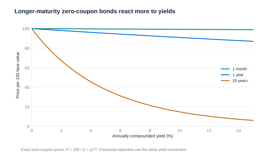
A single yield to maturity summarises the price of one instrument. It should not be mistaken for an assumption that every maturity in the market has the same discount rate. For more general fixed cash flows, valuation uses discount factors at each payment date; a yield to maturity is the single rate that reproduces the resulting total price under a chosen compounding convention.
Coupon bonds, par values and the term structure
A coupon bond distributes part of its value before the final redemption date. For annual coupons of amount , face value and an integer maturity , its single-yield pricing formula is
Each coupon and the principal must be discounted. When the coupon rate equals the required yield under the same payment convention, a conventional bond trades at par. A coupon rate below the required yield produces a price below par; a coupon rate above it produces a price above par. The discount or premium compensates the investor for the difference between contractual coupon income and the return required by the market.
| Annual coupon rate | Annual coupon | Calculated price | Price relative to par |
|---|---|---|---|
| 3% | 3 | 95.5482 | Below par |
| 4% | 4 | 100.0000 | At par |
| 5% | 5 | 104.4518 | Above par |
Under a nonflat term structure, the more general representation is , where is the cash flow at time and is the corresponding discount factor. A five-year annual-coupon bond can be treated as a portfolio of five zero-coupon claims: the first four pay coupons and the fifth pays coupon plus principal. This decomposition becomes important when different parts of the yield curve move by different amounts.
Macaulay duration as present-value-weighted timing
Macaulay duration measures the average time at which a bond's value is received, using present values as weights. Let be the present value of payment , let and define . Then
The weights sum to one for a positive-cash-flow bond, and duration is measured in years when payment times are measured in years. A ten-year zero-coupon bond has Macaulay duration ten years because all its value arrives at the final date. A coupon bond normally has a shorter Macaulay duration than its final maturity because some cash flows arrive earlier.
Portfolio duration is a market-value-weighted average under consistent conventions. Equal market-value investments in six-year and ten-year zero-coupon bonds give years of Macaulay duration. Equal face values would not generally give equal market-value weights. The distinction matters because risk sensitivity depends on today's economic values rather than simply the nominal amounts printed on the instruments.
The timing interpretation is particularly useful for relating assets to liabilities. Matching a portfolio's duration to the timing sensitivity of a future obligation can reduce first-order exposure to a small parallel rate change. It does not ensure that every cash flow occurs on the right date, eliminate reinvestment uncertainty under every rate path or provide protection against arbitrary changes in the curve's shape.
Modified duration and the value of a basis point
Modified duration converts cash-flow timing into first-order price sensitivity. For a nominal annual yield compounded times per year,
Here is the number of coupon or compounding periods per year, is expressed as a decimal annual rate, and is an absolute change in that rate. A rise from 4% to 5% is , not 1 and not a 25% relative yield change. The negative sign means that a positive-duration asset loses value when its yield rises.
One basis point, abbreviated bp, is 0.01 percentage points, or 0.0001 in decimal rate units. The positive magnitude of the approximate loss from a one-basis-point yield increase is often called PVBP, DV01 or the value of a basis point:
For the 20-year zero-coupon example at exactly 4.68%, and currency units per bp. A ten-basis-point rise therefore implies an approximate loss of 0.7654. Some systems report a signed PV01 sensitivity rather than a positive loss magnitude; the convention must be checked before combining positions or calculating hedge quantities.
Convexity and the limits of a linear approximation
Duration is the tangent slope of the price–yield relationship at the current yield. It becomes less accurate as the rate change grows because the slope itself changes. Price convexity, denoted , is the second derivative of price divided by price. A second-order approximation is
For a zero-coupon bond under annual compounding, . The 20-year example has convexity approximately 383.2850. For conventional positive fixed cash flows, convexity is positive: compared with the tangent approximation, the exact price is higher after either an upward or a downward yield shock. Duration alone therefore overstates the loss from a rise and understates the gain from a fall, for the same absolute shock.
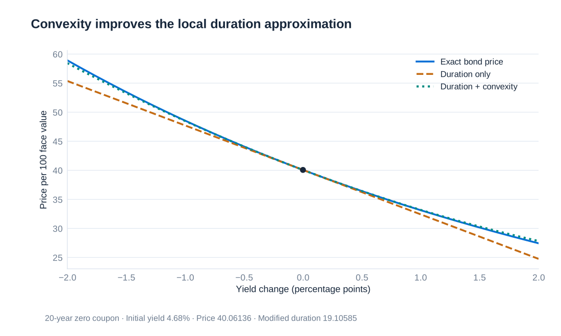
| Yield change | New yield | Exact repriced value | Duration approximation | Duration and convexity approximation |
|---|---|---|---|---|
| +0.01 | 5.68% | 33.124086 | 32.407300 | 33.175047 |
| −0.01 | 3.68% | 48.540051 | 47.715425 | 48.483171 |
The second-order calculation is considerably closer here but remains an approximation. Instruments with options can have different curvature because their expected cash flows change when rates change. Moreover, one duration and one convexity measure describe movement along one specified yield direction. They do not automatically capture twists, steepening or changes in credit spreads.
Hedging a bond portfolio with futures
Consider a corporate-bond portfolio worth USD 10 million with modified duration nine years. A one-basis-point parallel increase in its required yields produces an approximate value change of dollars. Suppose one long Treasury-bond futures contract loses approximately USD 90 for the corresponding one-basis-point increase. An offsetting hedge requires
The minus sign means 100 short futures contracts. If the matched rate movement occurs, the short futures gain approximately USD 9,000 while the bond portfolio loses approximately USD 9,000. This neutralises the specified first-order parallel-rate sensitivity. It does not make the entire portfolio risk-free or ensure zero profit and loss under all market changes.
Corporate-bond spreads can change relative to government yields; the portfolio and futures can have different convexity and maturity exposures; and the yield curve may move non-parallelly. The futures sensitivity can itself depend on delivery terms and the bond expected to be cheapest to deliver. Hedge ratios therefore require monitoring and rebalancing. Futures settlement also creates cash flows before bonds are sold, so sufficient liquidity is needed even when economic value changes offset.
Defining bond Value at Risk and the modelling horizon
Value at Risk, or VaR, is a selected quantile of a defined loss distribution over a defined horizon. If denotes a positive loss and is the confidence level, then . A 95% VaR is not a worst possible loss: the model assigns 5% of outcomes to losses exceeding that threshold. The cash flows, valuation date, holding period and treatment of carry must be stated.
Four simple methods can be illustrated with the same zero-coupon pricing function. One can model yield changes or directly model repriced bond changes, and one can use empirical quantiles or a normal-distribution approximation. These choices affect the result independently. A nonlinear pricing function can transform a symmetric yield distribution into an asymmetric price-change distribution.
| Method | Distribution assumption | Translation into loss |
|---|---|---|
| Historical yield quantile | Empirical distribution of yield changes | Adverse yield quantile multiplied by PVBP |
| Normal yield model | Normally distributed yield changes | Normal quantile, yield volatility and PVBP |
| Historical full repricing | Empirical yield scenarios applied to today's bond | Loss quantile from the repriced scenarios |
| Normal price-change model | Normal approximation to repriced price changes | Normal quantile multiplied by price-change volatility |
The numerical illustration uses weekly changes and therefore a one-week horizon. Mixing weekly volatility with a one-day VaR label changes the meaning of the result. The simple shock calculations below hold remaining maturity fixed while applying a yield change, isolating market-rate risk. A full one-week holding-period valuation should also reduce remaining maturity and include any cash flows or financing over the week; those adjustments must be applied consistently across all methods.
Historical yield shocks and the duration-based loss calculation
Suppose the empirical 95th percentile of weekly yield changes is an increase of 9.77 bp and the 5th percentile is −8.60 bp. For a long positive-duration bond, the upper yield tail is the adverse direction. Using the calculated PVBP gives
The equivalent duration calculation uses . The approximate fractional price loss is , or about 1.8666%. Multiplying by the price 40.061363 gives the same loss of approximately 0.748. Entering 0.00977 would mean a 97.7 bp shock and make the first-order loss ten times too large.
This estimate combines an empirical yield distribution with a linear value approximation. It is conditional on the selected historical period, data quality and quantile convention. A change in those inputs can change the result without any change in the bond itself. The relevant adverse tail would reverse for a short position, and a portfolio with options might not have a globally monotonic response to the same yield factor.
Normal yield shocks and full historical repricing
For a zero-mean normal model of weekly yield changes with standard deviation , the 95% first-order VaR is
With a weekly standard deviation of 5.443 bp, the result is currency units. The factor 1.645 is a one-sided 95% normal quantile; using 1.96 would instead correspond to a different tail probability. If a nonzero expected change is included, it must be carried through the loss model rather than silently omitted.
Historical full repricing avoids the duration approximation. For each observed or specified shock , calculate , then form the price change and loss . The following scenarios use yield changes expressed in bp; they are valuation calculations, not a claim that these few rows constitute the whole estimation sample.
| Yield shock, bp | Scenario yield | Scenario price | Price change |
|---|---|---|---|
| −5.0 | 4.630% | 40.4460 | +0.3846 |
| +2.3 | 4.703% | 39.8857 | −0.1756 |
| +5.1 | 4.731% | 39.6730 | −0.3884 |
| +4.0 | 4.720% | 39.7564 | −0.3049 |
| −3.1 | 4.649% | 40.2994 | +0.2380 |
| +13.1 | 4.811% | 39.0717 | −0.9896 |
| −1.0 | 4.670% | 40.1380 | +0.0766 |
| −6.2 | 4.618% | 40.5389 | +0.4775 |
| −3.7 | 4.643% | 40.3456 | +0.2843 |
| −1.8 | 4.662% | 40.1994 | +0.1380 |
| +1.7 | 4.697% | 39.9315 | −0.1299 |
| −2.9 | 4.651% | 40.2840 | +0.2226 |
| +8.5 | 4.765% | 39.4163 | −0.6451 |
| +6.2 | 4.742% | 39.5897 | −0.4716 |
| −8.2 | 4.598% | 40.6942 | +0.6328 |
| −11.8 | 4.562% | 40.9753 | +0.9140 |
| −1.7 | 4.663% | 40.1917 | +0.1303 |
| +4.8 | 4.728% | 39.6957 | −0.3656 |
| −13.5 | 4.545% | 41.1088 | +1.0474 |
| +5.8 | 4.738% | 39.6200 | −0.4414 |
For the same adverse 9.77 bp shock used in the linear model, full repricing gives . Positive convexity explains why this loss is slightly smaller than 0.747802. With a monotonic fixed-maturity price function, a consistently defined empirical upper yield quantile maps to the corresponding upper loss quantile, subject to the interpolation convention. One should not interpret a materially different value as a convexity effect without checking that the samples and signs match.
A normal model for price changes and numerical consistency
The fourth method estimates the standard deviation of repriced bond changes and then imposes a normal approximation directly on those changes. If their standard deviation is 0.417 currency units and their mean is neglected, the 95% VaR is . Yield-normal and price-normal models can give similar numbers for small shocks, but they are different assumptions because the bond price is a nonlinear function of yield.
An illustrative comparison based on weekly 2024 observations reports rounded VaR figures of 0.75 from the empirical yield quantile, 0.68 from the normal yield model, 0.66 from an empirical price-loss quantile and 0.69 from the normal price-change model. Its price-change summaries are a 5th percentile of −0.66, a 95th percentile of +0.72 and a standard deviation of 0.417. These are separate reported summary statistics, not enough information to reconstruct a complete common sample. In particular, the 0.66 empirical loss cannot be reproduced by applying the stated 9.77 bp adverse quantile to this fixed-maturity bond; the consistent calculation gives approximately 0.741.
The useful lesson is the method comparison, together with the requirement to reconcile inputs. A 95% loss quantile is the negative of the 5% price-change quantile, not the positive 95% price-change quantile. Small changes around 0.685 can also round to either 0.68 or 0.69 when underlying inputs have already been rounded. A robust calculation keeps unrounded prices and sensitivities, aligns observation frequency and sample dates, and applies a common loss convention before comparing model outputs.
Multiple yield-curve factors and instrument optionality
A coupon bond does not have only one economically relevant interest rate. Its component payments depend on discount factors at different maturities. Historical simulation can apply a joint observed change in the one-, two-, three-, four- and five-year rates to a five-year bond, then revalue all payments. The rate changes must come from the same historical observation so that their dependence is preserved.
For a first-order parametric model, let be a vector of decimal changes in the chosen curve rates, let contain the corresponding currency sensitivities , and let be the covariance matrix of those changes. Then
Adding separate maturity risks without covariance terms would miss the way curve movements reinforce or offset one another. Key-rate sensitivities make this structure visible. Similar valuation and scenario methods apply to interest-rate swaps and futures, with contract-specific cash flows and settlement conventions. Callable bonds, convertible bonds and bond options require additional modelling because exercise decisions or other risk factors can change the cash flows themselves.
Risk horizons, pull to par and a shrinking duration
A default-free zero-coupon bond pays its face value at maturity regardless of the path of interim market yields. As maturity approaches, its remaining duration falls and its price converges to that payment. Conditional on a similar distribution of yield shocks, its near-term interest-rate price sensitivity therefore decreases. This is a changing exposure, not a reason to apply the same volatility estimate mechanically at every future date.
If the horizon is exactly the maturity date, the nominal redemption cash flow is certain under the default-free assumption. The dispersion of that terminal payment due solely to interest-rate uncertainty is zero. It does not follow that every definition of investment loss or every investor's risk is zero: the comparison benchmark, purchase price, inflation and liquidity needs still matter. A coupon bond additionally creates reinvestment uncertainty for payments received before the horizon.
A short-term trader may need to know tomorrow's liquidation loss, whereas a saver concerned with retirement wealth in 2065 needs a model of cash flows and reinvestment over a much longer period. The horizon should follow the economic decision. Extending a short-horizon VaR by a square-root rule without considering declining maturity, changing sensitivities and cash flows can produce misleading results for bonds held over long periods.
Economic value of equity and the banking-book duration gap
Interest rate risk in the banking book, abbreviated IRRBB, concerns the effect of interest-rate movements on a bank's economic value and earnings outside its trading activities. Let and be the present values of assets and liabilities, and let be economic equity. If and are their modified durations under a common small parallel yield shock, then
The liability term must be subtracted because equity equals assets minus liabilities. A decline in the economic value of a liability benefits equity, other things equal, whereas a decline in asset value reduces it. Writing gives the equivalent expression .
For an illustrative bank with assets of 100, liabilities of 90 and equity of 10, take asset duration five years and liability duration zero. A parallel rise of 200 bp, or 0.02, gives , equal to the initial equity in magnitude. This is a first-order economic-value stress, not a statement that an accounting loss of exactly 10 must immediately be booked. If liability duration were two years instead, the approximate change would be .
Basel's IRRBB framework considers both economic-value and earnings measures and includes parallel and non-parallel interest-rate scenarios. A single 200 bp shock is useful for exposition and historical comparison, but it is not a complete modern stress framework. Steepening, flattening and movements concentrated at short maturities can reveal exposures concealed by a small aggregate duration gap.
Regulatory reference: Basel Framework SRP98, guidance on interest-rate risk in the banking book.
Deposit behaviour and historical evidence from German banks
The effective sensitivity of retail deposits is difficult to infer from legal maturity alone. A sight deposit can be withdrawn immediately, but a stable portion of aggregate balances may remain with the bank for years. At the same time, the rate paid to depositors may adjust slowly or rapidly when market rates change. Balance stability, contractual withdrawal rights and the repricing of deposit rates are related but distinct modelling questions. An average historical holding period is not automatically the correct duration.
Assuming a long behavioural duration for deposits can reduce the estimated duration gap against long fixed-rate assets. If customers withdraw funds, demand higher rates or move from sight deposits to time deposits during stress, that assumed protection can weaken. Behavioural assumptions must therefore be tested across scenarios and linked to the bank's funding strategy rather than accepted merely because past balances appeared stable.
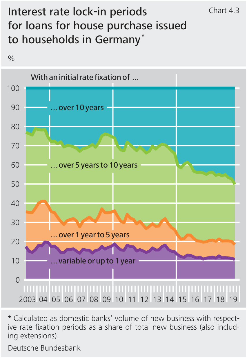
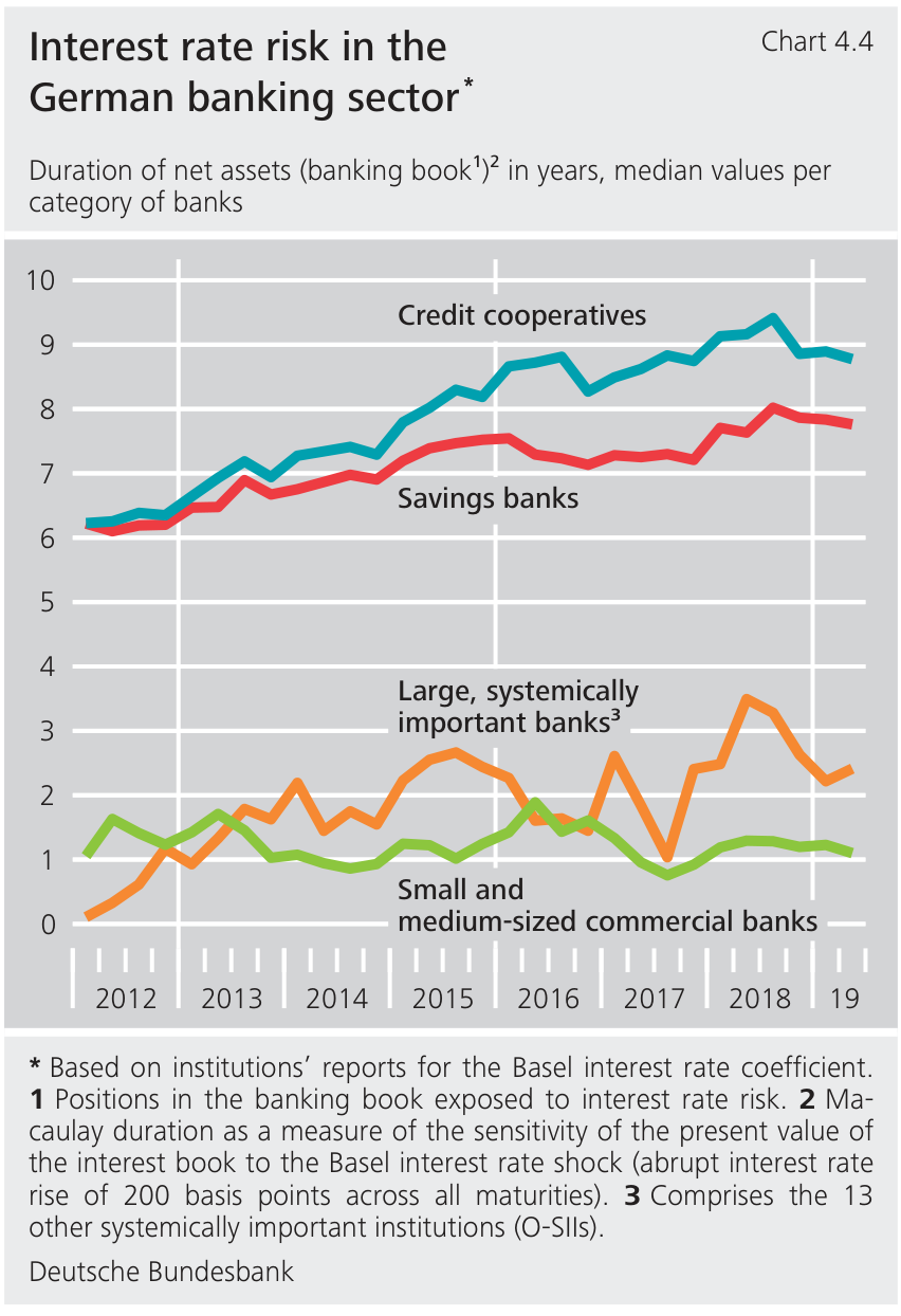
The historical German mortgage evidence shows a growing share of new household house-purchase lending with initial rate fixation longer than ten years during 2003–2019. The accompanying banking-sector measures show that duration exposure differed substantially across credit cooperatives, savings banks and commercial-bank groups. The composition of new loans is not identical to the duration of the whole existing balance sheet, but it helps explain how prolonged low-rate conditions could increase fixed-rate asset exposure.
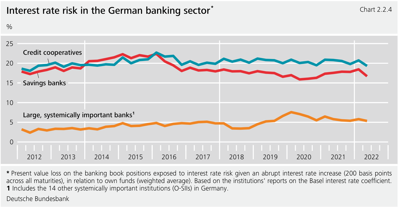
The Bundesbank's 2022 historical comparison expresses the present-value loss from a 200 bp upward shock as a percentage of own funds. Savings banks and credit cooperatives had larger reported ratios than the group of large systemically important banks in that series. These are category-level measures with specified weighting and reporting conventions, not the same as the loss rate on assets or a conclusion about every institution in each group.
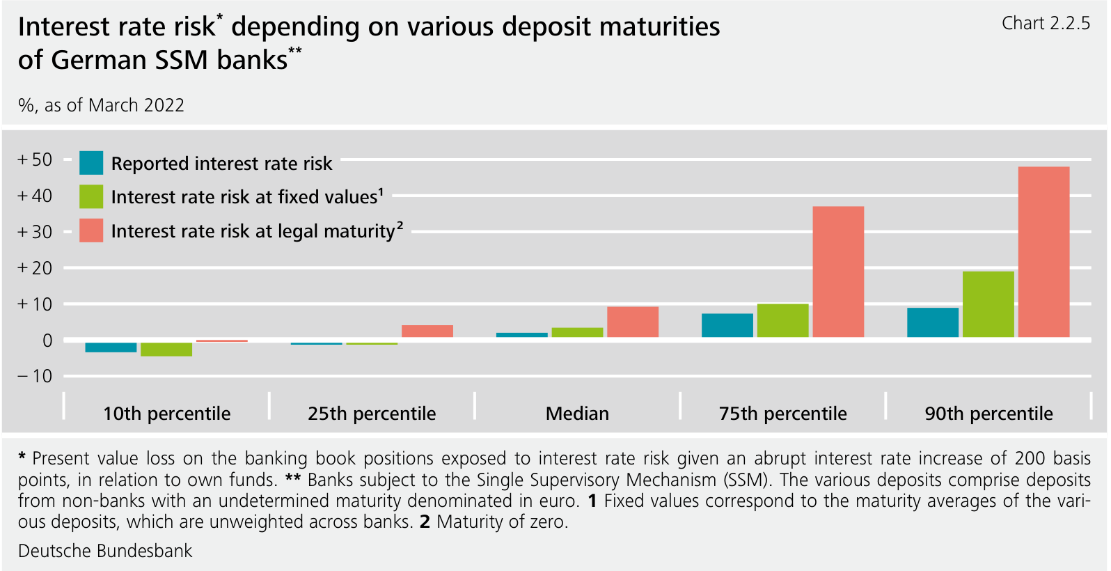
A separate March 2022 comparison for German banks under the Single Supervisory Mechanism contrasts reported deposit assumptions with fixed average maturities and legal maturity of zero for relevant nonbank euro deposits. The upper percentiles of measured risk rise substantially under the legal-maturity treatment. The comparison demonstrates model sensitivity: the economic-value estimate depends not only on observed market prices but also on assumptions about how deposit balances behave.
Repricing gaps and net interest income
Economic value is a present-value measure over future cash flows; net interest income, or NII, is interest revenue minus interest expense over a period. A bank can experience a fall in the market value of long fixed-rate assets while its current interest margin initially improves because some asset rates reset faster than deposit costs. Conversely, funding costs can increase before fixed asset income adjusts. The value and earnings perspectives are complementary, not interchangeable.
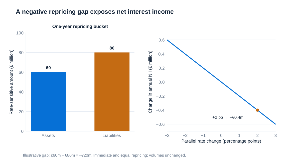
In a simplified one-period repricing model, let denote assets whose rates reset within the horizon and the corresponding liabilities. If both reprice immediately and fully to the same rate change, the approximate annualised income effect is
For hypothetical rate-sensitive assets of EUR 60 million and liabilities of EUR 80 million, the gap is EUR −20 million. A two-percentage-point increase implies an annualised NII change of million euros. Actual within-year effects depend on reset dates, rate pass-through, floors and business volumes. This gap is measured in currency and differs from the duration gap used to approximate economic-value changes.
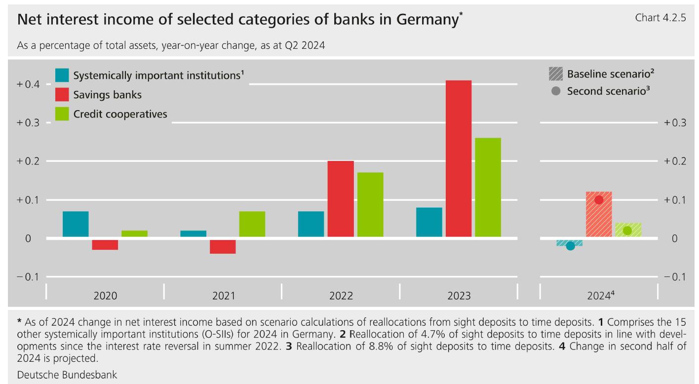
The Bundesbank's comparison through the second quarter of 2024 distinguishes realised annual changes in net interest income from scenario calculations for 2024. It shows stronger improvements for savings banks and credit cooperatives after the interest-rate reversal, while the projected effect depends on customers moving funds from sight deposits into more highly remunerated time deposits. Scenario bars should not be read as subsequently realised outcomes.
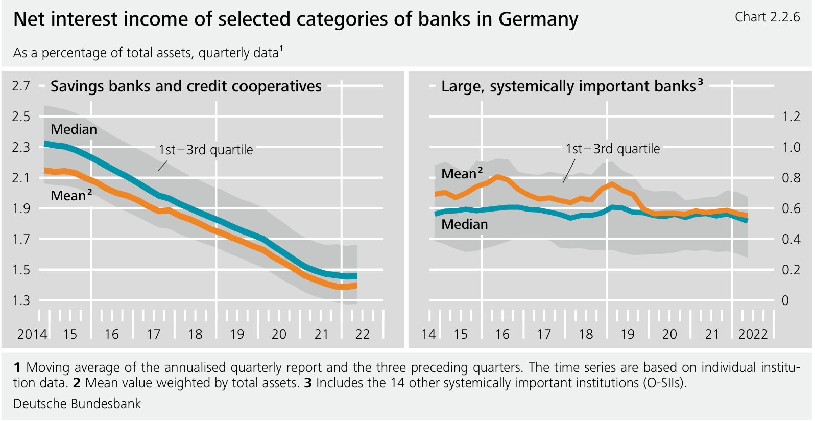
The longer 2014–2022 series shows declining NII relative to total assets for savings banks and credit cooperatives during much of the low-rate period. Large systemically important banks are shown on a separate scale and have different business mixes. The median, asset-weighted mean and interquartile range summarise different features of the distribution; comparing line heights without checking axes or weighting can give a misleading conclusion.
Amortised cost, hidden reserves and unrealised losses
Accounting carrying amounts and market values answer different questions. An instrument carried at amortised cost does not generally have its carrying amount reset to current fair value after every market-rate movement. Its economic value can nevertheless change materially. A market value above the relevant carrying value creates an unrealised gain, often described as a hidden reserve in this context; a market value below it creates an unrealised loss. Hidden reserves are not another name for losses.
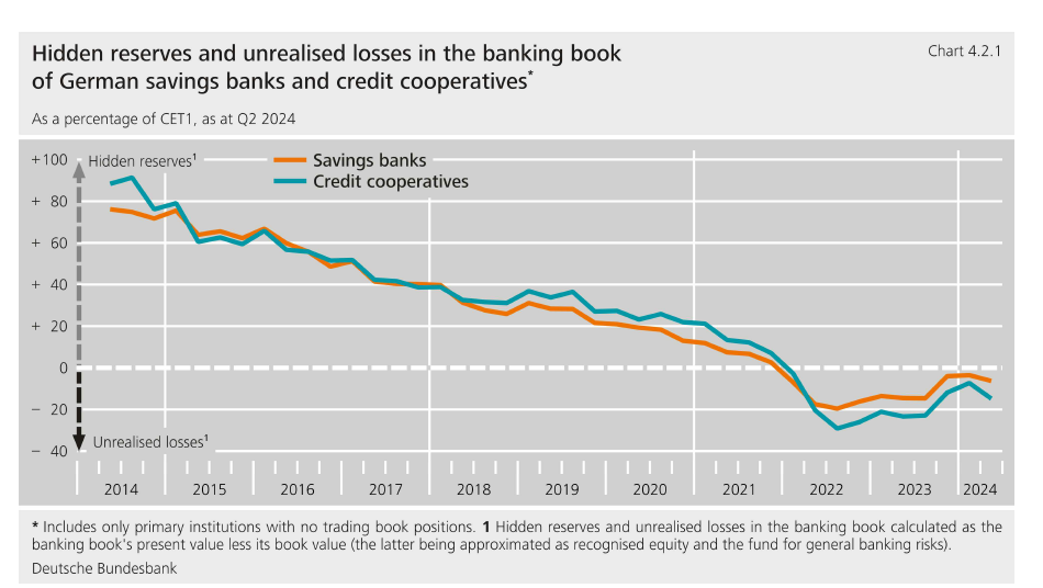
The historical Bundesbank series for German savings banks and credit cooperatives, expressed relative to Common Equity Tier 1 capital and extending to the second quarter of 2024, shows earlier positive differences turning negative around the 2022 rate increase. Its definition compares the banking book's present value with its book-value approximation. The chart illustrates a valuation gap under that stated methodology, not an automatic deduction of the whole amount from reported regulatory capital.
If a bank can hold assets and finance them as planned, an unrealised market loss need not require immediate liquidation. If deposits leave or collateral needs rise, sales can crystallise losses and reveal the connection between interest-rate risk and funding liquidity. Effective management therefore combines economic-value stress tests, earnings projections, behavioural deposit analysis and cash-flow capacity. The label “banking book” or “amortised cost” does not remove the underlying economic sensitivity.