
5. Option-Related Risks and Greeks
Market value, terminal payoff and profit
An option creates a contingent right rather than an unconditional obligation for its buyer. A call gives its holder the right to buy the underlying at the strike price; a put gives the right to sell. The writer receives the premium and accepts the corresponding obligation. Let denote the underlying price at time , the strike, the expiry date, and or the market value of a call or put. All prices and premiums in a particular example are expressed in the same currency per unit of underlying. Contract multipliers convert these unit amounts into the cash exposure of actual contracts.
The terminal payoff is the contractual amount received at expiry. Profit also accounts for the premium and, in a complete investment calculation, financing, transaction costs and any other cash flows. Unless stated otherwise, the terminal-profit examples below subtract the initial premium without accumulating interest. This convention makes the payoff geometry transparent; it is not a claim that financing is free in actual trading.
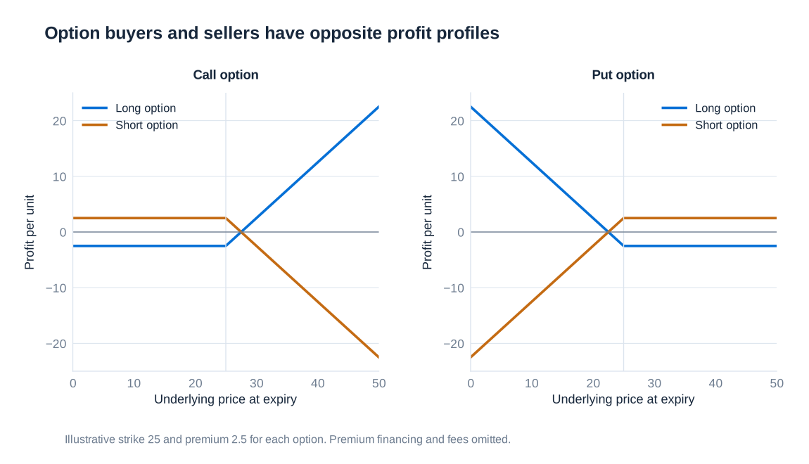
A call with strike EUR 25 purchased for EUR 2.50 can lose market value before expiry even while the underlying remains above EUR 25. Its resale price depends on the underlying, remaining time, implied volatility and interest rates. If the call expires with , its payoff is zero and the buyer loses the EUR 2.50 premium. If , it pays EUR 1 but the buyer still has a net loss of EUR 1.50. Ignoring financing, break-even is EUR 27.50. An option finishing in the money is therefore not necessarily a profitable investment.
Intrinsic value is the immediate-exercise value, for a call and for a put. The difference between market value and intrinsic value is conventionally called time value. For options with an immediate-exercise right it is non-negative under usual no-arbitrage conditions; for European options, discounting and exercise restrictions mean that comparison with immediate intrinsic value requires care. A positive remaining maturity should never be treated as guaranteeing a particular time-value sign for every contract.
| Position | Profit per unit | Maximum loss | Maximum profit |
|---|---|---|---|
| Long call | Unbounded if the underlying price has no upper bound | ||
| Short call | Unbounded if the underlying price has no upper bound | ||
| Long put | when | ||
| Short put | when |
Here and are premiums paid by buyers and received by writers; the put bounds assume a non-negative underlying price. For an underlying that can become negative, those bounds must be reconsidered. “Naked” describes an option position without the relevant offsetting exposure. A short call backed by shares has a different aggregate risk profile from a naked short call, even though the option leg itself is identical.
A bull call spread: constructing a bounded position
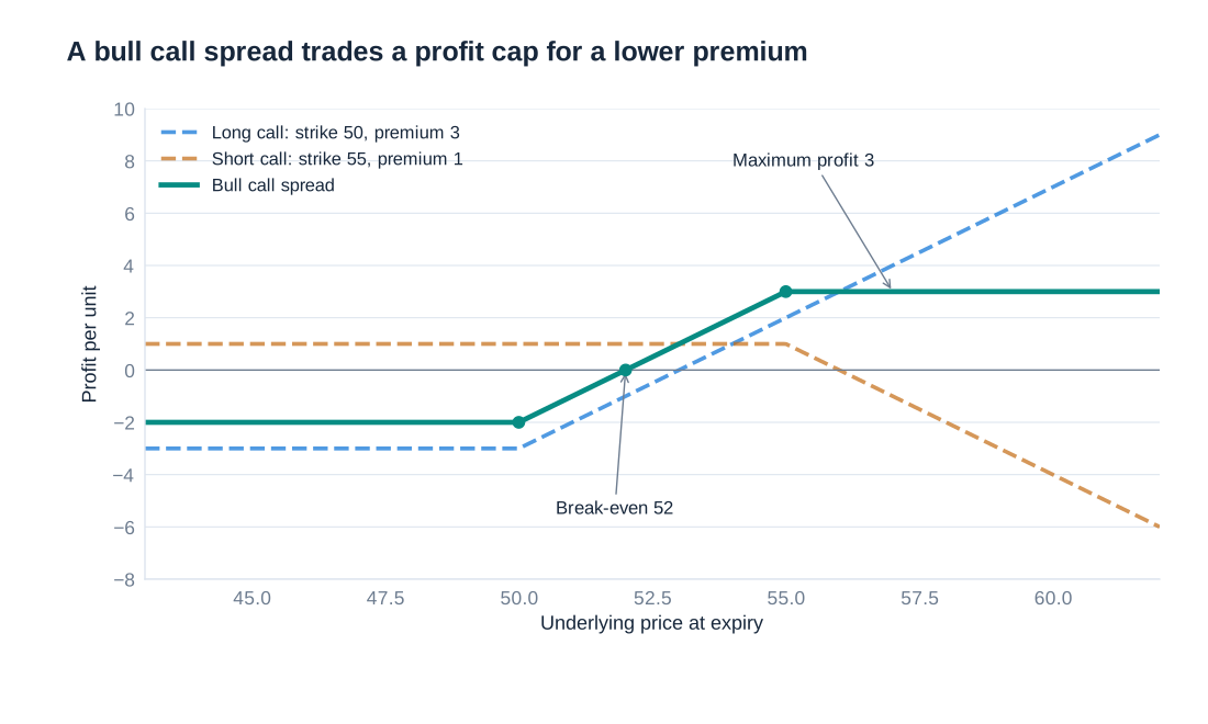
A bull call spread expresses a moderately positive view while limiting both the premium at risk and the benefit from a large price increase. Buy a call with lower strike and sell a call with higher strike , using the same underlying, expiry and unit quantity. If the premiums are and , the net premium paid is . The terminal profit is:
Consider a stock initially trading at USD 50. A strike-50 call costs USD 3, and a strike-55 call can be sold for USD 1. The initial debit is USD 2. Below the lower strike both calls expire worthless; between the strikes only the purchased call pays; above the higher strike the two exercise values rise at exactly the same rate, so their difference stops increasing.
| Terminal stock price | Long-call payoff | Short-call payoff | Net profit |
|---|---|---|---|
| USD 45 | USD 0 | USD 0 | −USD 2 |
| USD 50 | USD 0 | USD 0 | −USD 2 |
| USD 52 | USD 2 | USD 0 | USD 0 |
| USD 53 | USD 3 | USD 0 | USD 1 |
| USD 55 | USD 5 | USD 0 | USD 3 |
| USD 60 | USD 10 | −USD 5 | USD 3 |
The maximum loss is USD 2, the maximum profit is dollars, and break-even is dollars. The maximum payoff is USD 5, which differs from the maximum profit. These amounts are per unit: a spread using contracts covering 100 shares has a USD 200 initial debit and USD 300 maximum terminal profit, before fees and financing.
The terminal bound does not describe every operational exposure. If an American-style short call is assigned early, the investor may acquire a stock delivery obligation before the long call is exercised or sold. Funding, dividends and transaction costs can then affect realised results. The economic spread should be analysed together, while exercise and settlement obligations must also be managed leg by leg.
Equivalent shapes and the bull put spread
A bull put spread buys the lower-strike put and sells the higher-strike put. Its terminal option payoff is . This is the bull call spread’s payoff minus the constant . Consequently, the two option packages do not have identical raw cash payoffs. Their risk-dependent shapes are the same, with the difference accounted for by a fixed payment and the corresponding financing.
For European options with common maturity, put–call parity links their initial prices. With a constant continuously compounded rate , the call-spread debit equals the put-spread debit plus , taking the valuation date as zero. A matching risk-free cash position therefore converts one strategy into the other. Comparing only the names “calls” and “puts” conceals this equivalence; comparing only terminal profits without a financing convention can also conceal a genuine cash-flow difference.
At zero interest, the strike-50/55 call spread costing 2 corresponds to a bull put spread receiving a credit of 3. Below 50 the put spread pays −5, giving profit −2 after its initial credit; above 55 it pays zero and retains profit 3. The same break-even and maximum profit or loss follow. The example demonstrates why portfolio risk analysis must aggregate contractual cash flows and premiums before deciding whether a position is bullish, bearish or bounded.
Straddles, butterflies and the price of convexity
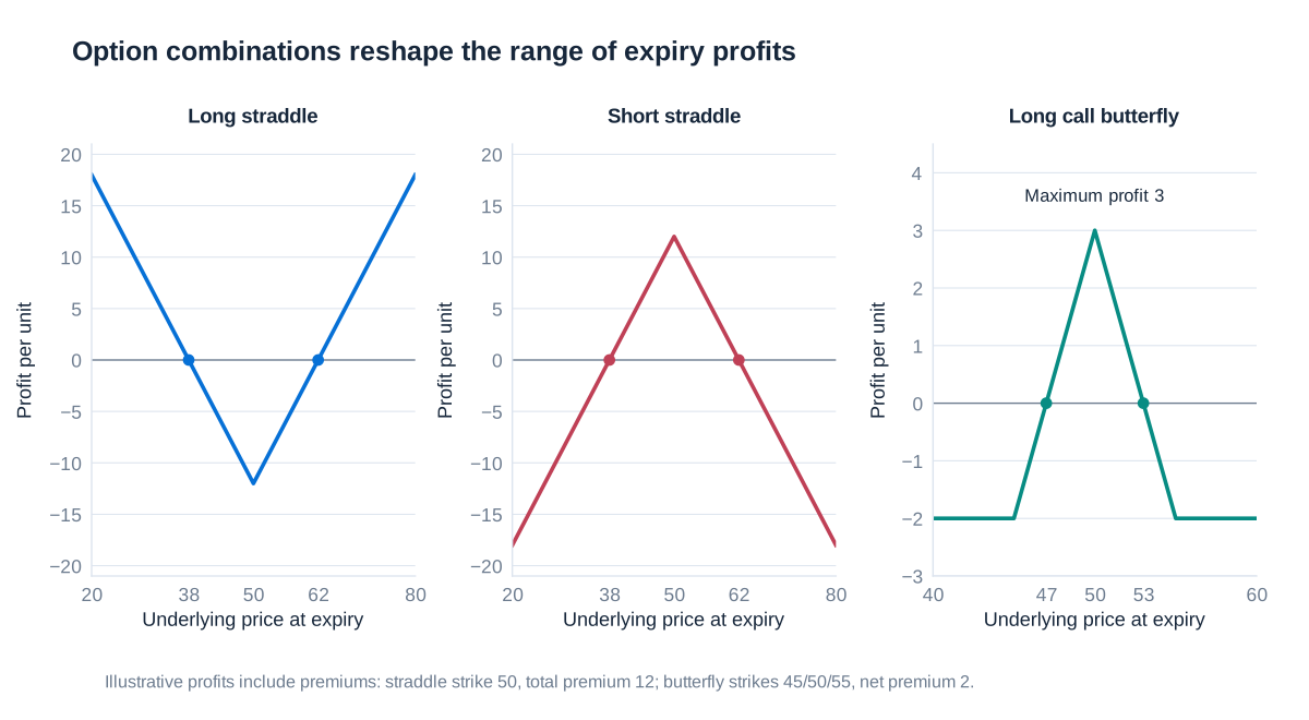
A long straddle purchases a call and a put with the same strike and expiry. Its terminal payoff is , and its profit is . The buyer benefits from a sufficiently large move in either direction, not merely from any movement. With total premium , break-even prices are and , provided the lower one is feasible for the underlying. The maximum loss is the premium, occurring when the terminal price equals the strike.
As an explicitly illustrative example, take and total premium 12. The break-even prices are 38 and 62. Expiry at 40 still produces a loss of 2 because the payoff of 10 does not recover the premium. Expiry at 70 produces profit 8. Before expiry, the value can increase when implied volatility rises even if the underlying price barely moves; an eventual terminal profit also depends on how much movement was already priced into the options.
A short straddle reverses these profits. The writer retains the total premium when the underlying finishes at the strike, but faces losses for sufficiently large moves. For a non-negative equity price the downside-price loss is bounded by , while the upside-price loss is unbounded. A calm historical sample can make this strategy appear attractive even though a rare large move creates severe losses. Margin calls can force liquidation before the terminal payoff is reached.
A long call butterfly buys one call at , sells two at , and buys one at , with equally spaced strikes and common expiry. Its payoff is:
The payoff is zero outside the two outer strikes and reaches at the middle strike. Subtract the net debit to obtain profit. With illustrative strikes 45, 50 and 55 and debit 2, the maximum loss is 2, maximum profit 3 and break-even prices 47 and 53. The purchased wings limit tail losses relative to an unprotected short-volatility position. Adding appropriate wings to a short straddle produces an iron-butterfly structure; a call butterfly is a related bounded structure, not literally a long straddle with two arbitrary extra options.
The Greeks as local sensitivities
Terminal diagrams hold the expiry date fixed and vary the final underlying price. Daily risk management asks a different question: how much will the current option value change when market inputs move? Write , where is annualised implied volatility, the relevant rate, and calendar time. A local Taylor expansion separates major sources of profit and loss:
| Greek | Definition | Interpretation |
|---|---|---|
| Delta | First-order value change per unit change in the underlying price | |
| Gamma | Change in delta per unit underlying-price change; determines local curvature | |
| Vega | Value sensitivity to implied volatility in the chosen volatility units | |
| Rho | Value sensitivity to the chosen interest-rate input | |
| Theta | Value change from calendar time passing, with other inputs held fixed |
The symbol is used both for a Greek and, when preceding a variable, for a change; the product means option delta multiplied by the price change. If instead time to maturity is the pricing input, calendar-time theta is . Confusing these conventions reverses the reported sign. A theta calculated per year must also be converted consistently before applying a one-day change.
Volatility of 20% is 0.20 in decimal form. An increase to 21% is one percentage point, meaning , not 1. A raw vega derivative of EUR 500 per unit decimal volatility implies approximately EUR 5 for that change. Trading systems often report vega directly per percentage point and rho per basis point or percentage point. Units must therefore accompany each number. FX options may require sensitivities to both domestic and foreign interest rates. If is the foreign rate, the expansion adds with . Complex portfolios need term-structure and volatility-surface buckets rather than one universal rate or volatility.
The expansion omits higher powers and cross-derivatives, including interactions between price and volatility. Its accuracy deteriorates for large shocks, near discontinuities and when important inputs are missing. Gamma improves on delta alone, but delta–gamma is still an approximation. Full revaluation under joint scenarios is the appropriate comparison when assessing whether the local approximation remains useful.
Aggregating Greeks into a usable risk report
Portfolio Greeks add across positions when they refer to the same risk factor, units and valuation conventions. For signed quantities and contract multipliers , portfolio delta is , and analogous expressions apply to the other Greeks. Long and short positions can offset in one sensitivity while reinforcing another. A near-zero aggregate delta is compatible with substantial gamma or vega exposure.
Consider an explicitly illustrative portfolio worth EUR 150 million with 120 positions in equities, indices and commodities. To make an aggregate scenario report interpretable, define a common parallel relative-price shock , a volatility shock , a rate shock , and elapsed time in days. These are standardised scenario coordinates, not claims that different underlyings always move together. The following local coefficients are in EUR millions:
| Sensitivity | Reported value | Meaning in the scenario approximation |
|---|---|---|
| Price delta | 10 | EUR 10 million first-order gain for a 1% parallel price increase |
| Price gamma | 2 | Second derivative with respect to ; contributes million |
| Vega | 5 | EUR 5 million gain per one-percentage-point volatility increase |
| Theta | −1 | EUR 1 million loss per day from time passing |
| Rho | 3 | EUR 3 million gain per one-percentage-point rate increase |
A 5% parallel price decline has : the delta contribution is −50 million and the gamma contribution is +25 million, giving a local delta–gamma estimate of −25 million. Reporting only −50 million is a first-order calculation, not a calculation that incorporates the stated gamma. A ten-percentage-point volatility increase gives a vega-only gain of 50 million, whereas a 10% relative increase from 20% to 22% volatility gives only 10 million. A half-percentage-point rate increase gives 1.5 million. These isolated calculations hold other inputs fixed; large joint stresses require full revaluation.
A practical report also separates underlyings, maturities and volatility buckets, identifies large concentrations, and shows the effect of proposed hedges. The number of positions and market value help describe scale but do not measure risk by themselves. Reporting a Greek simply as a currency amount without specifying its shock normalisation can produce errors larger than the apparent precision of the calculation.
Delta hedging and the residual gamma exposure
Suppose a purchased call has delta 0.6 and covers one share. A USD 1 increase in the share price gives an approximately USD 0.60 call gain. Shorting 0.6 shares creates an approximately USD 0.60 loss on the stock leg, cancelling the first-order effect. The hedge reverses for a short call: the writer buys shares. This is a local hedge at the current price, not a statement that all possible price movements now have zero consequences.
A trader short 100 calls on SAP, each covering one share and each with delta 0.6, has option delta −60. Holding 60 SAP shares makes combined delta zero. If each actual contract covers 100 shares instead, the required stock position is 6,000 shares. Contract-count and underlying-unit conventions must be reconciled before a hedge is executed.
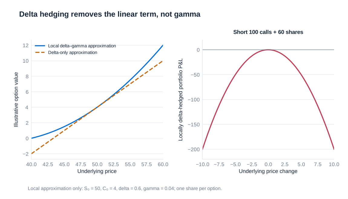
Shares have zero gamma, so they cannot remove the option position’s curvature. A short conventional call has negative gamma. In an explicitly illustrative local example, a long call’s value around is approximated by . The short-100-call portfolio plus 60 shares then has price-driven change:
A move of either +1 or −1 produces an approximate loss of 2 currency units; a move of either +5 or −5 produces an approximate loss of 50. The quadratic expression is a local approximation rather than a globally valid option price. It isolates gamma while ignoring theta, financing and volatility changes. A long option with an offsetting short stock position has the opposite local curvature.
After a rise in the underlying, a call’s delta may increase from 0.6 to 0.9. The short-100-call hedger must then raise the stock holding from 60 to 90 shares. After a decline, the hedger generally sells shares as delta falls. This buy-after-rises and sell-after-falls pattern explains the rebalancing burden of short gamma. Transaction costs, market jumps, discrete hedge intervals and illiquidity prevent a dynamic hedge from being an unconditional guarantee. Delta hedging also leaves volatility, rate, basis and model risks unless these are separately managed.
Fuel options: economic protection and cash expenditure
An airline purchasing fuel is exposed to rising fuel prices. Buying calls can cap the price paid while preserving the benefit of falling prices, at the cost of an upfront premium. Consider a simplified quarterly requirement of 100 barrels, hedged by calls on exactly 100 barrels with strike USD 25 and premium USD 1.20 per barrel. Assume the options settle when the fuel is purchased, the underlying exactly matches the fuel price and there are no financing or transaction costs.
| Fuel price per barrel | Physical purchase cost | Option receipt | Premium | Net expenditure |
|---|---|---|---|---|
| USD 20 | USD 2,000 | USD 0 | USD 120 | USD 2,120 |
| USD 25 | USD 2,500 | USD 0 | USD 120 | USD 2,620 |
| USD 40 | USD 4,000 | USD 1,500 | USD 120 | USD 2,620 |
Above the strike, the option receipt offsets every additional dollar paid for the matched fuel quantity. Below the strike the option expires, but physical fuel becomes cheaper. Calling the expired option a failed hedge ignores the combined position. The premium buys protection; it is not expected to be recovered in every state of the world.
Net cash expenditure is not automatically the same as an accounting-period expense. Fuel may first enter inventory, premiums may be paid earlier, and hedge accounting may defer or reclassify components. Nor does this simple example capture real jet-fuel basis risk when the hedge references crude oil, mismatched delivery dates or uncertain fuel volumes. An airline must evaluate the matched economic exposure and the residual mismatches separately.
Time value and reported earnings: the Lufthansa example
A purchased fuel call can gain intrinsic value as fuel prices rise while losing time value as expiry approaches or implied volatility falls. The total derivative value is the sum of these components, but accounting rules may recognise their changes in different places or periods. Under a historical IAS 39 cash-flow-hedge designation that separated intrinsic value from time value, the effective designated component could be deferred in other comprehensive income, or OCI, while excluded time-value changes entered profit or loss. OCI is part of comprehensive income and equity; it is not the same as current-period net profit.
For an illustrative accounting bridge, suppose the intrinsic-value component increases by EUR 575 million while time value decreases by EUR 289 million. The derivative’s net value rises by EUR 286 million, yet a qualifying intrinsic-value-only designation could show the 575 million effective gain in OCI and the 289 million time-value loss in profit or loss, before tax and other adjustments. These illustrative amounts describe the mechanism; they should not be confused with cash settlements, total airline profit or a verified quarterly financial statement.
Lufthansa’s 2011 annual report provides a documented historical example: it reported EUR 96 million of adverse changes in option time value in the financial result, primarily from fuel hedges, while realised fuel-hedging gains reduced fuel costs by EUR 694 million. These are full-year figures. The accompanying accounting policy distinguished changes in intrinsic value recognised in equity from changes in time value recognised in the financial result. The economic assessment therefore required both the fuel bill and the hedging components, not an isolated derivative expense.
The historical treatment should not be applied mechanically to current accounts. IFRS 9 provides cost-of-hedging treatment for qualifying excluded option time value, with recognition depending on the hedge and whether it relates to a transaction or a period. Lufthansa’s first-quarter 2018 report describes a change to the recognition of option time values on adoption of IFRS 9. Entities may also elect to retain IAS 39 hedge-accounting requirements under the applicable IFRS 9 policy choice. Designation, effectiveness, documentation and the specific hedged item therefore remain essential.
The risk-management lesson is to distinguish economic cash-flow protection, derivative fair-value changes and reported earnings. A hedge can meet its economic objective while creating accounting volatility; conversely, a smooth reported earnings series does not prove that all economic exposures are hedged. Risk reports should explain the reconciliation and the periods in which hedging gains, fuel costs and option premiums affect the accounts.
Accounting and case references: Lufthansa Annual Report 2011; Lufthansa Interim Report, first quarter 2018; IFRS 9 overview; IFRS 9, paragraph 6.5.15.