Econometrics Economics

What finite-sample theory asks

Finite-sample theory characterises estimators for a given n under precisely stated assumptions. It differs from asymptotic theory, which studies sequences of growing samples. In the familiar multiple regression y=Xβ+u, exact statements often condition on the observed matrix X. This is convenient for separating the stochastic properties of the disturbance from the realised variation in the regressors.

The core assumptions are a model linear in coefficients, a sampling mechanism with appropriate independence, no perfect multicollinearity and a zero conditional mean E[u|X]=0. The last assumption is the key to OLS unbiasedness; homoskedasticity and normally distributed disturbances are not needed for unbiasedness. However, unconditional mean zero E[u]=0 by itself is not sufficient because the error could systematically vary with the regressors.

Deriving conditional unbiasedness

Substituting y=Xβ+u into the OLS formula yields

If X has full column rank and E[u|X]=0, conditional expectation immediately gives E[β̂|X]=β. Taking expectations again proves E[β̂]=β. This proof is useful because it displays exactly where exogeneity enters: if E[u|X]≠0, OLS generally contains a systematic component dependent on regressors. Merely estimating a regression does not establish the assumption used to justify its result.

The conditional expectation assumption may fail when omitted variables correlate with explanatory variables, when economic agents jointly determine explanatory and outcome variables, or when a regressor is systematically measured with error. A regression can still compute the coefficient, but its expected value need not equal the structural parameter of interest.

Conditional covariance matrix of OLS

Allow the conditional covariance of the disturbance vector to be Ω=Var(u|X). Direct substitution gives

Under conditional homoskedasticity and no correlation across units, Ω=σ²I; the expression becomes

The ordinary estimated error variance is s²=RSS/(n−k−1) when the model has k explanatory regressors and an intercept. The denominator adjusts for the number of estimated parameters. Under the classical conditional assumptions, it is an unbiased estimator of σ². Usual standard errors take square roots of diagonal entries of s²(X′X)^-1.

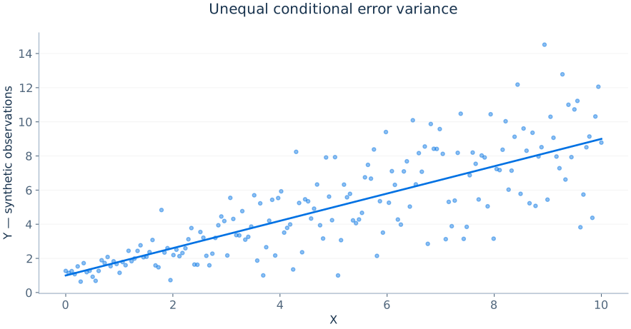
If the error variance differs across observations, these conventional standard errors can be inconsistent even when zero conditional mean ensures OLS is unbiased. Robust estimators are addressed separately because changing the variance calculation does not change the underlying estimated slope.

The Gauss–Markov theorem

Under the linear model, full rank, exogeneity and spherical errors (homoskedastic and uncorrelated disturbances), OLS is best linear unbiased (BLUE). "Best" means it has the smallest conditional covariance matrix among linear estimators unbiased for every value of β under the model; it does not mean OLS has the lowest variance among all imaginable nonlinear or biased estimators, nor does it require the disturbances to be normally distributed.

For intuition, consider any other unbiased estimator linear in y: β̃=Ay. Since unbiasedness requires AX=I, write A=(X′X)^-1X′+C with CX=0. Under Ω=σ²I, the difference between the competitors' covariance matrices is

Because CC′ is positive semidefinite, no linear unbiased competitor improves on OLS in the positive-semidefinite sense. The proof identifies exactly which assumptions deliver efficiency and why it may fail under heteroskedasticity or autocorrelation.

Sampling distributions under normal disturbances

If u|X is jointly normal N(0,σ²I), then β̂|X is normal with mean β and covariance σ²(X′X)^-1. Under this classical normal model, each t-statistic based on an appropriately estimated variance has an exact Student t distribution with n−k−1 degrees of freedom. For q linear restrictions, an appropriately constructed ratio of restricted versus unrestricted sums of squares follows an exact F distribution with q and n−k−1 degrees of freedom.

Without the normality assumption, OLS may remain unbiased and BLUE, while the conventional finite-sample t and F reference distributions are no longer exact. Researchers then commonly rely on asymptotic results and robust standard errors, or carefully justified resampling procedures.

Heteroskedasticity and finite-sample consequences

Heteroskedasticity means Var(u_i|X_i) changes with the regressors or other information. If E[u_i|X_i]=0 remains valid, coefficient unbiasedness can survive; the conventional variance simplification generally cannot. Homoskedasticity tests can sometimes describe variance patterns but are not necessary to justify using heteroskedasticity-robust covariance estimates. Robust standard errors must still be based on a correct independence, clustering or dependence structure.

Gauss–Markov assumptions in plain economic language

The linearity assumption concerns the parametrisation of the outcome's conditional mean, not the absence of nonlinear transformations of observed variables. Random sampling is a description of how economic units enter the dataset. No perfect collinearity requires variation in regressors that cannot be represented exactly by other included regressors. Zero conditional mean states that the excluded determinants do not change systematically with included regressors. Homoskedasticity states that, conditional on the regressors, the unexplained outcome variance is constant; no serial correlation requires distinct disturbances to be uncorrelated. Each assumption must be evaluated in the context of how the data were generated.

The Gauss–Markov claim concerns a particular benchmark class of estimators; it is not a universal claim that simple OLS dominates every alternative. With a known nonspherical covariance Ω, the generalised least squares estimator β̂ᴳᴸˢ=(X′Ω^-1X)^-1X′Ω^-1y may be more efficient when the model and covariance are correctly specified. Feasible GLS estimates Ω from data and therefore introduces additional sampling assumptions and potential sensitivity to covariance-model misspecification.

Homoskedasticity as a special case

For a binary outcome Y taking values zero and one, E[Y|X]=p(X) and Var(Y|X)=p(X)(1−p(X)). Unless p(X) is constant or takes special values, this conditional variance changes with X. A linear probability model therefore naturally exhibits heteroskedasticity even when the mean relationship is correctly approximated. This is a clear illustration of why robust standard errors are not an obscure remedy for rare statistical pathologies; heteroskedasticity often follows directly from the economic data structure.

Weighted least squares and what the weights mean

When the conditional variance is known to be proportional to a positive function h_i, dividing each observation’s equation, including the intercept, by √h_i makes the transformed disturbance homoskedastic. Weighted least squares therefore minimises squared residuals with weights w_i=1/h_i. A noisier observation receives less weight because it supplies less information about a common conditional-mean coefficient. W is the diagonal matrix of these positive weights.

Correct variance weights can improve efficiency under the maintained zero-conditional-mean model. Estimated weights give feasible WLS and require checking the variance specification; use a covariance estimator appropriate to the transformed estimating equations when that specification may be wrong. Precision weights are different from survey sampling weights or inverse-propensity weights, which address population representation or causal comparisons. In R, lm(y ~ x, weights = w, data = dat) expects inverse-variance weights for this precision interpretation. When the linear mean is only an approximation, weighting can change the population projection being estimated, so coefficient changes are not automatically evidence of improved causal identification.