Econometrics Economics

Why panels change the identification problem

Cross-sectional regressions compare different individuals, firms or regions. If units have enduring but unobserved characteristics, such as managerial skill, institutional quality or longstanding preferences, these factors may confound cross-sectional associations. Panel data repeatedly observe the same units and make it possible to remove fixed unobserved characteristics through within-unit comparisons. This advantage comes with new assumptions about time-varying confounding and dependence within units.

The canonical additive fixed-effects model is

Here α_i is a time-invariant unit effect, λ_t is a time effect shared across units, and u_it is the remaining time-varying disturbance. The coefficient β is identified by within-unit changes in X after adjusting for common time shocks under the relevant exogeneity assumptions. A variable that never changes within an individual cannot have its own slope separately identified in a model with unrestricted unit fixed effects.

First differencing with two periods

For two periods, start with Y_i1=α_i+βX_i1+u_i1 and Y_i2=α_i+βX_i2+u_i2. Subtract the first from the second:

The unobserved α_i disappears exactly. OLS on differences consistently estimates β when changes in X are appropriately exogenous with respect to changes in the disturbance. A constant unobserved individual characteristic need not be uncorrelated with X in levels, which is the key attraction of the method.

However, first differencing does not remove unobserved time-varying factors. If a firm changes investment because an unrecorded demand shock raises its expected sales, that shock may affect both ΔX and ΔY. Measurement error can also become more important after differencing because signal in a persistent variable is reduced while measurement noise remains.

Fixed-effects (within) estimation

For more than two periods, take each individual's time average. The model Y_it=α_i+βX_it+u_it implies Ȳ_i=α_i+βX̄_i+ū_i. Subtract the average equation from each period:

OLS on these demeaned data estimates the within-unit slope. An equivalent least-squares dummy variable estimator includes an intercept for each unit except an omitted reference, when feasible. Both estimators remove additive time-invariant α_i and yield the same slope under corresponding specifications.

The standard assumption for the static FE model is often strict exogeneity: E[u_it|X_i1,…,X_it,…,X_iT,α_i]=0 for every t. This requires every disturbance u_it to have mean zero conditional on the entire regressor history, including future X values. In particular, it rules out feedback in which a shock today changes next period’s regressor; it is stronger than the sequential exogeneity sometimes used in dynamic time-series models. A lagged dependent variable with fixed effects creates additional complications in short panels.

Unit and time fixed effects

Adding λ_t adjusts for common shocks or trends affecting all units. A two-way fixed-effects regression with unit and time dummies is

In the absence of other controls, β compares changes within units relative to the corresponding changes in other units that identify the regression. Two-way FE can be a useful descriptive control strategy, but under staggered policy adoption and heterogeneous dynamic treatment effects, its coefficient need not equal a transparent, convex weighted average of treatment effects. Modern difference-in-differences methods may be preferable for such designs.

Difference-in-differences

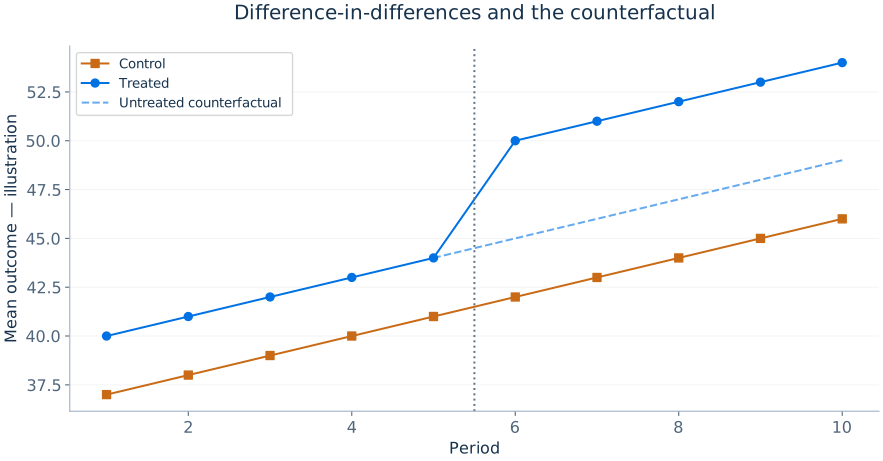
With treated and control units observed before and after a policy, the basic DID estimator is

The critical parallel-trends assumption says that, without treatment, treated and control units would have experienced the same expected change in the outcome over the comparison period. This is about unobserved counterfactual changes; pre-policy trends can provide useful evidence but cannot logically prove the counterfactual assumption for the post-policy period.

Random effects and correlated random effects

A conventional random-effects model treats the individual effect as uncorrelated with explanatory variables, allowing a weighted combination of within- and between-unit information. When this exogeneity holds, RE can be more efficient than FE. When α_i correlates with X, standard RE can be inconsistent while FE can remain consistent under its own assumptions. A correlated random-effects or Mundlak specification includes unit-level means of time-varying regressors to model the dependence between α_i and X. Such formulations can connect FE and RE and provide meaningful additional parameters in certain settings.

Model choice is not settled solely by a mechanical Hausman test. The assumptions, the effects of interest, whether time-invariant regressors matter and the clustering structure all deserve attention.

Serial correlation and clustered inference

Observations from the same unit over time are rarely independent. A FE regression usually requires standard errors clustered by unit, under a large-cluster asymptotic framework and assumptions of independence across clusters. If shocks are also correlated across units at a date, the dependence may require additional adjustment or a different inferential strategy. Unbalanced panels are often estimable, but attrition related to unobserved potential outcomes can affect interpretation.

library(fixest)
fe <- feols(y ~ x1 + x2 | firm_id + year, data = dat,
            vcov = ~ firm_id)
summary(fe)
# A DID specification when policy adopts at a common date:
did <- feols(y ~ treated:post | firm_id + year,
             data = dat, vcov = ~ firm_id)
summary(did)

A worked fixed-effects transformation

Suppose two regions are observed in three years, and the researcher wants to estimate the relationship between policing and crime. The first region has a permanently higher baseline crime level because of unmeasured historical conditions; the second region has permanently lower baseline crime. A pooled regression may confuse these fixed differences with policing if police resources are also systematically higher in the first region. Region fixed effects subtract each region's own mean from outcomes and regressors, leaving only deviations within that region over time.

This procedure does not make an increase in policing exogenous. If a region hires extra police in anticipation of a crime wave, the within-region policing change may still correlate with the unobserved impending shock. A stronger source of identification might be a funding formula, a predetermined staffing shock or another externally motivated policy change. Fixed effects remove fixed confounding, not policy responsiveness.

Clustering and effective information in panels

Repeated observations on the same region or firm share unobserved influences, so a regression with thousands of firm-year rows but only 20 firms may have less independent information than the raw row count suggests. The level of clustering should reflect the assignment and shock mechanisms. If a reform is assigned at the region level, clustering at an individual worker level is usually inadequate because treatment variation and shared shocks occur at the region level. If both region and year shocks exhibit complex dependence, more sophisticated inference may be needed.

Treatment timing, cohort effects and event-time comparisons

Let G_i denote the first period in which unit i is treated. The group-time effect ATT(g,t) compares the average outcome at date t for the cohort first treated in g with its counterfactual outcome if it had remained untreated. This target allows the effect to differ across cohorts and with exposure duration. Identification needs an appropriate parallel-trends assumption, no anticipation over the specified window, suitable overlap and an untreated comparison group.

For example, a cohort treated in 2023 can be compared in 2024 with units still untreated in 2024, if those units provide a credible counterfactual. Units treated in 2022 are already exposed; using them as controls can subtract their evolving treatment effects. Cohort-time estimators make this comparison explicit before aggregating. Event time e=t−g measures duration since adoption, whereas calendar time t locates common shocks. Aggregation should disclose cohort weights and which cohorts remain observed at each horizon. Non-rejection of pre-treatment differences supports a limited diagnostic; it does not establish parallel counterfactual trends after treatment.