Econometrics Economics

Prediction with many potential regressors

The number of available predictors may become large relative to the number of observations. Advertising campaigns, consumer purchases and macroeconomic forecasts can be described by hundreds of covariates and lags. An unrestricted OLS regression can fit training data extremely closely yet produce poor out-of-sample performance because its coefficients respond to sampling noise. Regularisation deliberately introduces bias to reduce variance and potentially improve prediction.

A predictive model and a causal model are judged by different criteria. A useful predictor need not cause an outcome: it may simply be an early or correlated signal. For example, web searches may help forecast sales without being a manipulable determinant of consumption. A well-designed causal estimate instead requires a defensible counterfactual comparison, often with a carefully structured adjustment set.

Bias–variance trade-off

For a new observation with covariates X₀, a predictive estimate ŷ(X₀) has mean squared error composed of squared bias, variance and irreducible outcome noise under suitable conditioning. Increasing model flexibility can reduce approximation bias but increase estimation variance. A very complicated model may capture idiosyncratic patterns in the training sample that do not recur in fresh observations. Shrinkage aims to control that trade-off.

Ridge regression

Ridge minimises the OLS loss plus a squared-coefficient penalty:

The intercept is usually left unpenalised and the explanatory variables are standardised before fitting. The tuning parameter λ≥0 controls the amount of shrinkage: λ=0 recovers OLS under full rank; larger λ moves slope coefficients toward zero. For centred X and Y, the matrix form is β̂ʳⁱᵈᵍᵉ=(X′X+λI)^-1X′y. Ridge stabilises near-collinear designs but typically does not set individual coefficients exactly to zero.

Lasso and sparse models

Lasso replaces the squared penalty by the absolute-value penalty Σ|β_j|, enabling variable selection through exact zero coefficients. When a relatively small number of predictors carry most of the useful signal, Lasso can give a compact forecasting model. It is not automatically superior to ridge: highly correlated blocks of predictive variables can lead to unstable selection, while ridge may distribute coefficient weight more smoothly. Elastic net combines L₁ and L₂ penalties and can be valuable when many correlated predictors are present.

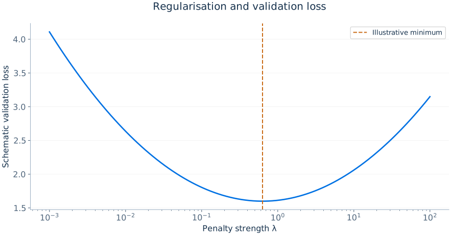
The tuning parameter is not estimated from ordinary OLS t-statistics. It is commonly chosen to minimise cross-validated prediction loss. Choosing both the variable transformations and the penalty by repeatedly checking the same test sample leads to evaluation leakage. A genuine holdout dataset should remain unused until final evaluation.

K-fold cross-validation

Divide the training sample into K folds. For each candidate λ, fit the model on K−1 folds and predict observations in the held-out fold. Average the holdout losses across folds and choose a penalty with satisfactory cross-validated performance. Finally refit on the entire training sample and evaluate once on an untouched test set. Nested validation or a separate validation stage may be helpful when many hyperparameters and model families are compared.

Principal components

Principal component analysis transforms a vector of correlated regressors into orthogonal linear combinations ranked by the amount of predictor variance they explain. If the standardised data matrix is X, the principal-component directions solve an eigenvector problem for X′X or the corresponding covariance matrix. A prediction model can regress Y on a limited number of leading components. This may reduce dimensionality, but the components explaining most variation in X do not necessarily explain most variation in Y, so the number of components should be selected for the predictive task.

Time-series prediction with many predictors

Macroeconomic forecasting may employ many correlated series such as employment, confidence, production, prices and financial indicators. Dynamic factor models assume that much of their joint variation reflects a smaller number of latent factors. Factor-based forecasts can reduce estimation complexity while exploiting a wider information set, but data revisions, changes in relationships and future-data leakage complicate evaluation.

Simple implementation in R

The following schematic example assumes complete data and numeric predictors with identical names and order in train and test. glmnet standardises predictors internally by default. With factors, build the test matrix using the training terms, factor levels and contrasts, then verify identical columns; two separate model.matrix calls alone do not guarantee compatible encoding. Use the same prespecified folds to compare ridge with Lasso, and keep test outcomes out of every tuning decision.

library(glmnet)
X <- model.matrix(y ~ . - 1, data = train)
y <- train$y
set.seed(2026)
fold_id <- sample(rep(seq_len(10), length.out = nrow(X)))
ridge <- cv.glmnet(X, y, alpha = 0, foldid = fold_id)
lasso <- cv.glmnet(X, y, alpha = 1, foldid = fold_id)
coef(lasso, s = "lambda.min")
newX <- model.matrix(y ~ . - 1, data = test)
stopifnot(identical(colnames(X), colnames(newX)))
pred <- as.numeric(predict(lasso, newx = newX, s = "lambda.min"))
sqrt(mean((test$y - pred)^2))

Ridge shrinkage and singular values

Let the centred design matrix have singular value decomposition X=UΣV′. Ordinary least squares in its principal directions multiplies components of the outcome by the reciprocal of singular values. When a singular value is very small, tiny fluctuations in the outcome can create large coefficient changes. Ridge modifies the contribution by replacing the unstable inverse weighting with factors σ_j/(σ_j²+λ), damping directions with weak predictor variation. This explains why ridge often performs well with collinear economic indicators.

The penalty λ should be selected on training data, and model assessment should use genuinely new observations. Inference on individual ridge or Lasso coefficients is not obtained by reading conventional OLS t-statistics off a selected model; the regularisation bias and selection stage require specialised methods.

Choosing prediction tools for a specific task

Use simple OLS when predictors are few, relationships are approximately linear and extrapolation or interpretation is important. Consider ridge when many predictors are correlated and forecasting dominates variable selection. Consider Lasso when a sparse predictive representation is plausible and a compact specification is valuable. Principal components may help when many indicators share a few latent factors; dynamic factor models extend this intuition to time-dependent macroeconomic panels.