
6. Nonlinearities, Logs and Interactions
Flexible conditional means with coefficients that remain interpretable
Linearity in parameters versus linearity in regressors
The classical least-squares formula estimates models linear in the unknown coefficients, not necessarily linear in the original data variables. A model with X2, log(X), a treatment interaction or year indicators remains linear in parameters if these transformed regressors enter additively with linear coefficients. Conversely Y=exp(β0+β1X)+u is nonlinear in parameters and cannot be estimated as written by ordinary linear least squares without changing the model and error assumptions.
Functional form choices impose substantive statements about marginal effects. Adding a polynomial is not a purely cosmetic technique: it says that the relationship may bend in a systematic way. Using logs can create a proportional-effect interpretation, handle substantial skewness and express economic elasticities. A model must still be checked for sensible predictions, influential observations and any new restrictions imposed by the chosen transformation.
The main logarithmic models
For positive Y and X, four common forms are useful. Level–level: Y=β0+β1X+u has a constant β1-unit marginal change in Y. Log–level: ln(Y)=β0+β1X+u has approximately a 100β1-percent change in Y per unit X. Level–log: Y=β0+β1ln(X)+u has an approximate β1/100-unit change in Y per 1% increase in X. Log–log: ln(Y)=β0+β1ln(X)+u has constant elasticity β1, so a 1% increase in X corresponds to approximately a β1% difference in Y.
| Form | Specification | Coefficient meaning |
|---|---|---|
| Level–level | Y = β0 + β1X + u | Y units per X unit |
| Log–level | ln Y = β0 + β1X + u | ≈ 100β1 % Y per X unit |
| Level–log | Y = β0 + β1ln X + u | ≈ β1/100 Y units per 1% X |
| Log–log | ln Y = β0 + β1ln X + u | Exact elasticity of the exponentiated log predictor: β1 |
When the dependent variable is logged, exponentiating the fitted conditional mean of ln(Y) does not generally reproduce E[Y|X]. Jensen's inequality implies that E[exp(log Y)|X] is not simply exp(E[log Y|X]). Forecasts in original units may require a retransformation or smearing correction, especially with heteroskedastic log residuals.
Quadratic and higher-order terms
A quadratic specification is
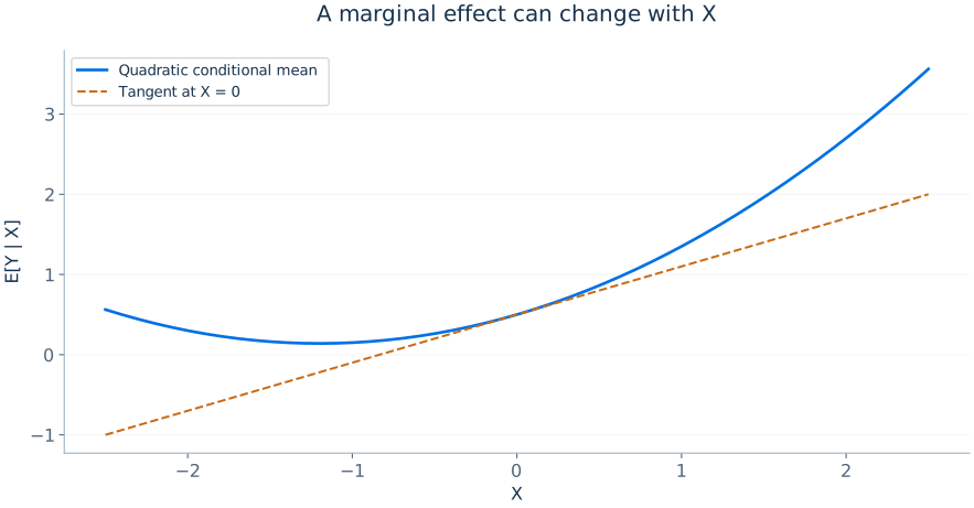
Its marginal effect is β1+2β2X. If β2<0, the function is concave and a positive β1 may eventually turn into a negative marginal effect. The turning point is X*=−β1/(2β2), if β2≠0. One should report whether this point falls inside the observed data range before interpreting it economically. Arbitrarily high-degree polynomials may overfit, fluctuate sharply near boundaries and extrapolate poorly.
Interactions between two continuous regressors
Let E[Y|X,Z]=β0+β1X+β2Z+β3XZ. Holding Z fixed, the marginal effect of X is
The coefficient on X describes its effect at Z=0, which may lie outside the substantively interesting range. Centering Z around its mean makes β1 refer to the average observed level of Z, improving interpretability. The interaction coefficient measures how X's marginal effect changes per unit increase in Z; its sampling uncertainty and the covariance between estimates matter when computing standard errors for a particular marginal effect.
Binary × continuous and binary × binary interactions
The model E[Y|D,X]=β0+β1D+β2X+β3(DX) permits different slopes in treated and untreated groups. For D=0 the slope in X is β2; for D=1 it is β2+β3. The treatment-control contrast at X=x is β1+β3x, not simply β1. The standard error of this contrast uses Var(β̂1)+x2Var(β̂3)+2xCov(β̂1,β̂3).
With two binary variables A and B, adding A×B allows the group possessing both characteristics to differ from the sum of their separate main effects. In a fully interacted model with two binary indicators, fitted means match the four group-specific means. This is an example of a saturated linear model. The same algebra underpins the simplest difference-in-differences specification discussed in the panel-data chapter.
Flexible regression and partial interpretation
A statistical model can flexibly approximate the conditional mean without identifying a causal mechanism. Adding many transformations does not eliminate omitted confounders or endogeneity. An estimated nonlinear regression also requires evaluating the relevant marginal effect at economically appropriate values, accompanied by uncertainty intervals, rather than declaring the coefficient on the original term to be the whole effect.
The multivariate marginal-effect formula
For a smooth conditional mean m(x)=E[Y|X=x], the marginal effect of Xj is ∂m(x)/∂xj. For a discrete or binary treatment, derivatives can be inappropriate; instead calculate the change in predicted outcome between treatment states, holding the remaining covariates fixed. Average marginal effects average unit-specific partial effects across the observed sample; marginal effects at the mean evaluate a nonlinear function at a particular artificial covariate vector. These quantities differ because nonlinear functions do not generally commute with averaging.
If m(X)=β0+β1X+β2X2, the derivative β1+2β2X is individual-specific. The average marginal effect is β1+2β2X̄ in this quadratic case, but more complex functions may require averaging calculated effects over all observations. When models contain multiple interacted covariates, state exactly which are held constant and where the derivative is evaluated.
Inference for turning points and elasticities
The turning point of a quadratic, X*=−β1/(2β2), is a ratio of estimated coefficients. If β2 is imprecisely estimated near zero, this ratio can have a highly skewed distribution; the standard delta method may be unreliable. A graph of the estimated function with confidence bands often communicates uncertainty more responsibly than reporting a single turning-point value. For a predicted effect L(β̂) involving multiple coefficients, incorporate the entire estimated covariance matrix.
Consider a log–log model with estimated slope 0.75 and robust SE 0.12. A simple 95% interval for the elasticity is approximately 0.75±1.96(0.12), or (0.515,0.985). This interval characterises sampling uncertainty in the coefficient under the model, not whether a policy-induced price change has the same effect as a historical market association.
From log predictions to outcomes in original units
A fitted log model describes m(x)=E[ln(Y)|X=x]. Its exponent exp(m(x)) is a conditional geometric mean, and is a conditional median when the log disturbance has conditional median zero. To obtain the conditional arithmetic mean, write Y=exp(m(X))exp(u) and average the second factor conditional on X. The resulting correction can vary across covariate values; exponentiation alone generally understates the conditional mean.
If u conditional on X is normal with constant variance σ2, the correction is exp(σ2/2). With a constant error distribution but without normality, a smearing estimate uses the sample mean of exp(ûi). A single global smearing factor is generally insufficient when the distribution of u changes with X. For example, if m(x)=2 and σ2=0.25, exp(2) is about 7.39 but the conditional mean is exp(2.125), about 8.37. Multiplicative comparisons between two covariate values cancel the correction only if it is identical at those values.
Binary outcomes: linear probability, logit and probit
For a binary outcome, the conditional mean is a probability. A linear probability model uses p(x)=x′β and interprets a coefficient of 0.04 as a four-percentage-point change, holding other regressors fixed. The model is simple but can predict below zero or above one, and its error variance p(x)[1−p(x)] is generally heterogeneous.
Logit uses the logistic distribution function Λ and probit uses the standard normal distribution function Φ. Both keep fitted probabilities between zero and one. With independent observations, maximum likelihood chooses coefficients to maximise the Bernoulli log-likelihood shown below, where pi is the fitted probability and yi is zero or one. A logit coefficient describes a change in log odds, not a percentage-point change. For an untransformed continuous regressor without interactions, its probability marginal effect is βjpi(1−pi); the probit analogue is βjφ(xi′β), where φ is the standard normal density. For binary regressors, compare predicted probabilities at zero and one and average these differences if the estimand is an average effect. These models still require a credible identification argument for causal claims.
| Model | Probability function | Main interpretation |
|---|---|---|
| Linear probability | x′β | Slope in probability units; use a suitable robust covariance |
| Logit | Λ(x′β) | Slope in log odds; calculate probability contrasts |
| Probit | Φ(x′β) | Slope on the normal index; calculate probability contrasts |