Econometrics Economics

Parameters and estimators

A parameter is a fixed feature of a population distribution; an estimator is a random variable because it changes across samples. The bias of θ̂ is E[θ̂]−θ, and unbiasedness means its expectation equals the parameter. Consistency means the estimator approaches the parameter in probability as the sample expands; these are not equivalent properties. An estimator can be biased in small samples and still be consistent, or unbiased under particular conditions and yet have unacceptably high variance.

Mean squared error (MSE) combines bias and sampling variance:

A mildly biased estimator can have smaller MSE than an unbiased alternative. This is a major rationale for shrinkage methods in prediction. For causal estimation, however, we must carefully distinguish sampling MSE from identification bias: shrinking a coefficient cannot repair a bad instrument or confounding by unobserved variables.

Sampling distribution of the average

For an independent sample with finite variance σ², E[Ȳ]=μ and Var(Ȳ)=σ²/n. If the underlying observations are normally distributed, the sample mean is exactly normal for any n. Otherwise it is often approximately normal in sufficiently large samples by the CLT. A sampling distribution is an imagined distribution across repeated datasets drawn by the same mechanism; one normally observes only one dataset and estimates the resulting uncertainty.

The estimated standard error SE(Ȳ)=s/√n is itself random. When errors are normally distributed and σ² is unknown, (Ȳ−μ)/(s/√n) follows a Student t distribution with n−1 degrees of freedom. The tails approach standard normal as the degrees of freedom increase. Where the normal assumption is implausible, a large-sample normal approximation can remain useful, subject to the CLT and a trustworthy variance estimator.

Confidence intervals

A 95% confidence interval is a random interval procedure whose coverage probability is 95% under the assumed model and repeated sampling. It is not, in classical frequentist terminology, a statement that there is a 95% probability that a fixed realised interval contains the fixed parameter. An approximate interval is

For a small normal sample with unknown variance, the multiplier is usually the appropriate t critical value instead of 1.96. Intervals must use a variance estimator consistent with the data design. Independence-based confidence limits will often be too narrow with positively correlated observations.

Hypothesis testing

A statistical test uses an estimator's sampling distribution to evaluate whether observed evidence is compatible with a null hypothesis. For H₀: θ=θ₀, the familiar statistic is

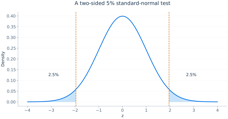
A p-value is the null probability of obtaining a test statistic at least as extreme as that observed, as defined by the alternative. It is neither the probability that H₀ is true nor the probability that the alternative is correct. A 5% two-sided test rejects for sufficiently extreme positive or negative t values; a one-sided test assigns the rejection region to one tail in advance.

There are at least three distinct standards for discussing an estimate: statistical significance, economic magnitude and identification quality. A coefficient can be statistically distinguishable from zero while too small to matter economically. Conversely, a large estimated policy effect might have a wide confidence interval because the independent sample is small. Neither pattern alone proves causality.

Comparing two population means

For independent samples from groups A and B, the difference in sample means Δ̂=Ȳ_a−Ȳᵦ estimates the corresponding difference in population means. If the groups are independent, an estimated standard error allowing unequal variances is

Pooling group variances is not necessary unless the equal-variance model is explicitly justified. If the observations instead come in matched pairs or repeated measures on the same units, the covariance between observations changes the variance formula; treating pairs as independent wastes information or understates uncertainty.

Error sources that confidence intervals do not fix

The standard error accounts for sampling variation under the chosen sampling model. It does not automatically account for coding errors, biased measurement, selective publication, misspecified dynamics, omitted confounders or invalid instruments. Confidence intervals quantify one part of uncertainty: they do not certify the validity of the economic interpretation. This separation becomes essential as methods become more sophisticated.

The bootstrap and its correct scope

A nonparametric bootstrap repeatedly samples observations with replacement from the observed empirical distribution, recomputing the estimator for each pseudo-sample. The resulting distribution of bootstrap estimates approximates the estimator's sampling distribution under suitable conditions. Percentile, basic and studentised bootstrap intervals can differ, particularly when distributions are skewed. Bootstrapping should follow the data-generating structure: resample clusters rather than individual students if the statistical units are classrooms, and use appropriate time-series block schemes when observations are serially dependent.

The bootstrap is not a universal solution to identification or weak-instrument problems. Resampling a confounded observational dataset reproduces its confounded association; it does not recreate an ideal experiment. Standard bootstrap procedures can also fail for nonsmooth estimators and nonregular parameters. A resampling method must be validated for the estimator and sampling scheme in use.

Type I and Type II errors

A Type I error is rejection of a true null. For a correctly calibrated 5% test, its probability under the null is 5%. A Type II error is failure to reject a false null; power is one minus the Type II error probability for a specified alternative. These probabilities vary with sample size, population variance, the size of the genuine effect, and the testing design. A 5% significance threshold is not a substantive guarantee that a published claim is likely true.