
5. Multiple Regression and Partial Effects
The ceteris paribus interpretation, regression anatomy and multicollinearity
Why multiple regression is necessary
Economic outcomes rarely respond to a single observed determinant. Workers with more education also tend to differ in experience, sector, location and family circumstances. A regression of wages on education alone incorporates all dimensions correlated with education into the same slope. Multiple regression attempts to describe the association of wages with education while holding selected other characteristics fixed. Write
Here each βj describes the change in the conditional linear predictor of Y associated with a one-unit increase in Xj holding the other regressors fixed. This phrase is an interpretation of a mathematical conditional comparison, not a guarantee that such a comparison can be made for the observed population or that βj represents a causal effect.
For example, suppose annual earnings are related to schooling, experience and industry. An education coefficient in this model refers to workers of equal included experience and industry. If ability is unmeasured and affects both schooling and earnings, the education coefficient can still be biased. More variables are not always better: conditioning on mediators of an effect or on colliders may create new biases rather than remove confounding.
How OLS solves the multiple-regression problem
The OLS estimator minimises the sum of squared residuals over all k+1 coefficients. With an n×(k+1) design matrix X, an n-vector y and coefficient vector β, the model and least-squares objective can be written as
Differentiating gives the normal equations X′Xβ̂=X′y. If X has full column rank, the unique solution is
The matrix X′X encodes variation and correlations among regressors; X′y encodes their covariation with Y. Full column rank rules out exact linear dependencies and requires at least as many rows as parameters. Positive residual degrees of freedom additionally require n>k+1; statistical independence is a separate sampling assumption. It is not the same as assuming the explanatory variables are mutually uncorrelated: strongly correlated regressors can be estimated, although with lower precision.
A projection matrix Px = X(X′X)-1X′ satisfies ŷ=Pxy, while residuals are û=(I−Px)y. The projection makes the residual vector orthogonal to every included regressor, X′û=0. These expressions reveal the geometric interpretation of OLS as projection onto the column space of X.
The Frisch–Waugh–Lovell theorem
The Frisch–Waugh–Lovell (FWL) theorem gives an intuitive recipe for understanding β̂1. First regress X1 on all other included explanatory variables and save its residual r1. Second regress Y on those same other variables and save residual rᵧ. Finally regress rᵧ on r1 without an additional intercept. The slope equals β̂1 from the full multiple regression:
The coefficient uses variation in X1 that cannot be linearly predicted by the other regressors. If education is almost perfectly predicted by age and occupational controls, little independent variation remains for identifying its slope. FWL also explains why adding controls can alter an estimate: the relevant variation in X1 is redefined, not simply the number of residual degrees of freedom.
For partialling out it is mathematically valid to residualise Y and X1 on the other controls. It is not generally enough to residualise Y alone, because the denominator and the covariance must correspond to the adjusted variation in X1. The two-residual procedure provides a practical diagnostic and is especially useful in high-dimensional nuisance-adjustment methods.
The omitted-variable bias formula
Suppose the true conditional model includes both X and Z:
If Z is omitted, the population simple-regression slope of Y on X satisfies
This exact population formula isolates two ingredients: the omitted variable must affect the outcome (β2≠0) and correlate with the included regressor (Cov(X,Z)≠0). The sign of the bias is the product of these two signs. If ability increases earnings and is positively related to education, omitting ability tends to bias upward the observed schooling association, although the sign and size of actual ability bias are empirical questions.
The formula has a multiple-regression generalisation: replace X by its residual after projection on other included controls, and measure the covariance between this residual and the omitted variable. A variable unrelated to the regressor after appropriate controls cannot induce conventional omitted-variable bias in its coefficient, even if that omitted variable is important for explaining Y.
The dummy-variable trap and qualitative regressors
Dummy variables encode a categorical characteristic. A model with an intercept and three mutually exclusive industry categories normally includes only two dummies, leaving the third as reference. Including all three creates exact multicollinearity because the intercept is the sum of the three indicators. The omitted reference category is not ignored: it is represented by the intercept, and the included dummy coefficients compare groups with that reference group, conditional on other regressors.
Changing the reference category changes the reported dummy coefficients but not fitted values. For a categorical variable with multiple levels, reporting the estimated mean outcomes or explicit pairwise contrasts can be more illuminating than interpreting arbitrary base-category coefficients individually.
Multicollinearity and precision
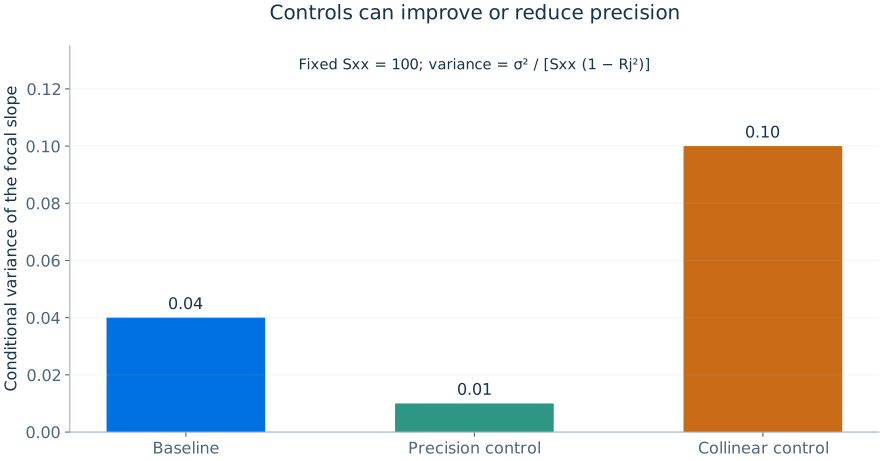
Imperfect multicollinearity means regressors are strongly but not perfectly related. OLS coefficients remain computable, but their variance grows because the residual variation in a particular regressor is limited. Under homoskedasticity,
where Rj2 is obtained by regressing Xj on the other regressors. The variance inflation factor VIFj=1/(1−Rj2) summarises the inflation relative to orthogonal regressors. A large VIF signals reduced precision, not automatically bias or a need to delete economically necessary controls. Whether a variable is appropriate must be decided using the research design.
Scaling, standardisation and interpretation
Standardised variables replace an observed regressor by its deviation from the sample mean divided by its sample standard deviation. If both Y and Xj are standardised, the slope expresses outcome standard deviations per one standard-deviation increase in Xj, holding other regressors fixed. Standardising Xj alone leaves the coefficient in original Y units per standard deviation of Xj. They can facilitate comparisons of association but should not substitute for effects in economically meaningful units. Scaling and centering change intercepts and selected slopes under interactions; they do not create identification.
Consider the fitted model log(wage)=β0+β1educ+β2exper+β3exper2+u. The predicted percentage effect of another year of education is approximately 100β1%, while the marginal change in log wages with respect to experience is β2+2β3exper and varies with experience. Reporting β2 alone as a constant marginal effect is incorrect.
Confounding, precision controls and bad controls
A useful distinction separates controls that protect causal identification from variables that mainly improve precision. A pretreatment variable related to both treatment and outcome can reduce confounding when the conditional-independence assumption is plausible. A baseline variable strongly predictive of outcome but unrelated to random treatment can reduce residual variance and therefore improve precision. A post-treatment variable can instead remove part of the very effect of interest and must not be included automatically. Good modelling chooses controls based on economic timing, institutions and causal logic rather than applying a universal 'include everything' rule.
For example, suppose education affects occupation, which affects wages. When seeking education's total effect, controlling for occupation can block an important causal pathway and produce a different estimand. If occupation is also influenced by unmeasured factors that affect wages, conditioning may create additional bias. A researcher interested in education's direct effect not mediated by occupation requires an alternative estimand and stronger assumptions, not a casual reinterpretation of the same regression coefficient.
Interpreting a full regression table
A carefully interpreted regression table reports coefficient units, explanatory variables, sample size, R2 or comparable fit measure, fixed effects if any and a clear standard-error method. When a coefficient changes after adding controls, several explanations remain possible: omitted confounding in the earlier specification, changes in the analysed sample due to missing control variables, altered weighting implicit in the regression, interactions or functional misspecification. To isolate the effect of controls, compare specifications on a common estimation sample whenever possible.
A policy coefficient can remain nearly constant when controls are added, but coefficient stability alone does not verify exogeneity: all models may omit the same unobserved confounder. Conversely changes across well-justified specifications should trigger substantive inquiry rather than mechanical selection of the coefficient with the smallest p-value.