
14. Time Series, AR Models and Forecasting
Dependence over time, stationarity, lag selection and honest forecasting
The nature of time-series variation
A time series is an ordered sequence of observations indexed by time, such as quarterly GDP, monthly inflation or daily asset returns. Unlike independent cross-sectional observations, adjacent observations often contain overlapping information: output today depends on yesterday's output, price levels inherit past changes and financial volatility can persist across periods. Statistical inference and prediction must account for this temporal structure rather than mechanically using formulas derived for independent observations.
A useful transformation is the first difference ΔYt=Yt−Yt₋1. For a positive series, Δln(Yt)=ln(Yt)−ln(Yt₋1) approximates the growth rate between t−1 and t. If Y is an index or total price level, a difference may be meaningful in level units, whereas a log difference measures a proportional change. Transformations can remove some forms of trend but can also change the economic question and introduce their own serial-correlation pattern.
Autocovariance, autocorrelation and stationarity
For a weakly stationary process, the mean E[Yt]=μ is time-invariant, the variance is finite and constant, and the covariance between Yt and Yt₋k depends only on lag k, not on the date t. Denote this autocovariance γ(k)=Cov(Yt,Yt₋k). The autocorrelation is ρ(k)=γ(k)/γ(0). Positive first-order autocorrelation means that observations above the mean tend to be followed by further observations above the mean.
Nonstationary time series may have changing means, changing variance or persistent stochastic trends. A series displaying visual trend is not automatically a unit-root process; the distinction between deterministic and stochastic trends is important for transformations, hypothesis tests and forecast uncertainty.
The autoregressive model of order one
An AR(1) process has the form
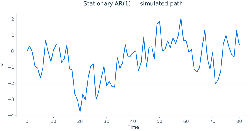
where εt has conditional mean zero given information available at t−1. With |φ|<1 and white-noise innovations of variance σ2, the causal stationary solution has mean μ=c/(1−φ) and variance σ2/(1−φ2). These stationary moments apply when the process is initialised in its stationary distribution; an arbitrary initial value creates a transient. Conditional mean zero, which is stronger than simple lack of correlation with the past, justifies the conditional forecast below. For positive φ less than one, a shock gradually decays instead of disappearing immediately.
The k-step conditional forecast with known parameters is
Forecasts tend toward the long-run mean as k increases when |φ|<1. If φ approaches one, shocks decay very slowly and long-horizon uncertainty becomes substantial. At φ=1, the process is a random walk with drift: standard stationary AR formulas no longer apply.
Autoregressions of higher order
An AR(p) model includes p lags of the dependent variable:
Higher lag orders allow richer persistence but add parameters and require a larger effective estimation sample. The relevant stability condition for AR(p) concerns the characteristic polynomial's roots, not merely whether each estimated coefficient individually has absolute value below one. The regression can be estimated by OLS under appropriate exogeneity of lagged predictors with respect to the current innovation and additional stationarity or regularity assumptions.
Model selection: AIC, BIC and validation
The lag order p can be chosen with information criteria that balance fit and model complexity. A common Gaussian-style form using a residual-variance estimate is
where kp counts fitted parameters and T is the effective sample size. Lower criterion values are preferred for the candidate set under the selected convention. BIC's penalty grows with ln T and more strongly favours parsimonious models as samples expand. For valid comparisons, lag candidates should be evaluated on comparable estimation samples and criteria must use compatible normalisations.
Time-series cross-validation should preserve chronological order. One strategy is rolling-origin evaluation: estimate using data available up to date t, forecast t+1, move forward and repeat. This provides a practical estimate of performance under genuine future prediction. Random-fold cross-validation can leak future information if the folds break temporal structure.
MSFE, forecast uncertainty and benchmarks
For h-step forecasts Ŷt₊h|t, forecast errors are et₊h=Yt₊h−Ŷt₊h|t. Mean squared forecast error is MSFE=(1/m)Σe2 over genuine evaluation dates. A good benchmark may be a historical average, random walk or simple AR model. Sophisticated models should be judged against credible simpler alternatives using data not employed in estimation.
Forecast intervals require accounting for innovation uncertainty, parameter uncertainty and possible model instability. In a stationary AR(1) with known φ and innovations having constant conditional variance σ2 and zero conditional mean, the k-step innovation forecast-error variance is
Longer horizons ordinarily accumulate uncertainty. If the model parameters are estimated, additional uncertainty must be considered when the sampling scale makes it material.
Unit roots and spurious regression
A random walk Yt=Yt₋1+εt has a unit root and is not weakly stationary. Regressing one unrelated trending series on another can produce apparently impressive t-statistics and R2 values even though the underlying innovations are independent—a spurious regression. Unit-root tests have nonstandard reference distributions and should not be interpreted like ordinary regression t-tests. Differencing can recover a stationary process in some cases, but differencing a genuinely stationary trend-adjusted relationship can discard valuable information.
When two nonstationary series share a stable long-run equilibrium relationship, they may be cointegrated. An error-correction model can represent both short-run changes and adjustment toward the long-run equilibrium. This is a substantial extension; simply finding a statistically significant regression between two price levels is insufficient evidence of cointegration.
Practical forecasting in R
The following illustrates AR fitting, time-aware training and basic diagnostic thinking. Real research should check seasonal effects, residual autocorrelation, structural breaks and forecast stability.
# Assume y is a numeric time-series vector ordered chronologically.
y_train <- head(y, length(y) - 12)
y_test  <- tail(y, 12)
fit_ar <- arima(y_train, order = c(1, 0, 0), include.mean = TRUE)
fc <- predict(fit_ar, n.ahead = 12)
rmse <- sqrt(mean((y_test - fc$pred)^2))
print(rmse)
acf(residuals(fit_ar))Dynamic effects and distributed-lag models
An economy may not respond fully to a policy in the same period it occurs. A distributed-lag model describes the outcome as a function of current and lagged explanatory variables, such as
Here δ0 is the contemporaneous response holding other explanatory terms fixed, while δ1 and δ2 capture further responses at later horizons under the model's timing interpretation. If a permanent one-unit increase in X persists from period t onward, the cumulative response after all included lags have taken effect is δ0+δ1+δ2. The standard error of this sum must include covariances among lag-coefficient estimates.
For causal interpretation, the input sequence X must be exogenous in a sufficiently strong sense relative to unobserved shocks. Lagging a regressor does not automatically eliminate endogeneity: agents may anticipate shocks, policies may respond to past disturbances and persistent unobserved conditions may correlate with present values of X.
Forecast comparison and structural breaks
A structural break occurs when the mean, variance or predictive coefficients change. An AR model fitted entirely before a major reform can forecast poorly afterward even with low historical residual error. Rolling evaluations and stability tests are therefore central to forecast reliability. A model can have excellent one-step forecasts but deteriorate at longer horizons because small dynamic errors accumulate. Always report the horizon, training window and forecast benchmark; claiming a forecasting model is “accurate” without these details is incomplete.
Testing for a unit root: the null hypothesis matters
The augmented Dickey–Fuller regression explains the first difference using a lagged level, optional deterministic terms and lags of the first difference. In the equation below, the unit-root null is γ=0. The stationary alternative has a negative adjustment coefficient in the appropriate stable specification. The constant, trend and lag order influence the reference distribution and the interpretation; an ordinary Student t critical value is inappropriate.
Failure to reject a unit root does not prove its presence, especially in short or highly persistent series. Conversely, the KPSS test starts from a stationarity null, so its p-value answers a different question. Conflicting results should prompt examination of structural breaks, deterministic trends and finite-sample power, rather than a majority vote between tests. Too much differencing can introduce unnecessary serial correlation and remove economically meaningful level relationships. In R, tseries::adf.test includes a constant and linear trend by default; this choice should be understood rather than mistaken for a neutral test of every possible deterministic specification.
| Test | Null hypothesis | Meaning of rejection |
|---|---|---|
| ADF | Unit root under the specified deterministic terms | Evidence against that unit-root model |
| KPSS | Level or trend stationarity, depending on specification | Evidence against that stationarity model |