
2. Probability for Economic Data
Random variables, joint distributions, conditional expectations and sampling
Random variables and distributions
A random variable assigns a numerical value to each possible outcome of an uncertain process. Discrete random variables possess a probability mass function p(x) = P(X=x), and their probabilities sum to one. Continuous random variables are represented by a density f(x): probabilities correspond to areas under the density, not to its value at a single point. The cumulative distribution function F(x)=P(X≤x) exists for both types and is nondecreasing.
An economic variable often has a skewed distribution: earnings, wealth and firm size can have a long right tail. A sample mean describes average income, while a median can convey the experience of a typical observation more effectively. Neither statistic alone characterises dispersion or the differences between population subgroups.
Expectations, variance and covariance
The expected value is the probability-weighted average of possible outcomes. For a discrete variable it is E[X] = Σx x p(x); in the continuous case E[X] = ∫x f(x)dx, whenever the integral exists. Linearity makes expectations especially useful:
Unlike linearity of expectations, independence is required for some convenient simplifications of variance. The population variance is Var(X)=E[(X−μx)2]=E[X2]−μx2, with standard deviation σx = √Var(X). Variance is measured in squared units; standard deviation returns to the scale of X. For constants a and b, Var(a+bX)=b2Var(X).
Covariance measures signed joint variation:
The correlation coefficient ρx𝓏=Cov(X,Z)/(σxσ𝓏) is dimensionless and lies between −1 and 1. Correlation zero rules out a linear association but not all nonlinear dependence. Independence implies zero covariance when moments exist, but zero covariance does not generally imply independence. For example, if X is symmetric about zero and the required moments exist, X and its square X2 can be uncorrelated while X2 is completely determined by X.
The variance of a sum is
If covariance is negative, combining variables can reduce risk. This is the statistical foundation of portfolio diversification; independent variables have zero covariance, but the useful variance formula does not itself require independence.
Conditional expectations and the law of iterated expectations
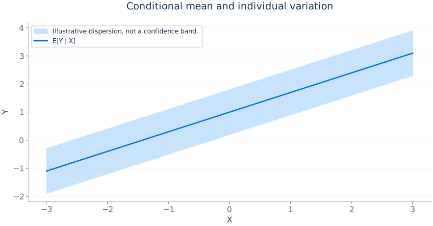
The conditional expectation E[Y|X=x] is the average value of Y among observations with X=x in the population distribution. It is a function of x, not a constant. For the income–consumption relationship, it describes average consumption at different income levels. The conditional expectation function (CEF) is the unrestricted mean relationship, while a linear regression will approximate this relationship using a linear combination of regressors.
The law of iterated expectations states
One can obtain the overall average by first averaging Y within groups defined by X and then averaging those group means using the groups' population probabilities. Define ε=Y−E[Y|X]. By construction E[ε|X]=0, and ε is uncorrelated with every integrable function of X. This exact decomposition does not require that the CEF be linear.
The law of total variance refines this decomposition:
Its first component measures variation in conditional means across X and its second measures average variation within the X groups. This helps explain regression fit as the division between predicted and unexplained variation.
Conditional independence
If Y and D are conditionally independent given X, knowledge of D adds no information about the distribution of Y once X is known. For causal inference, the stronger requirement is often that the vector of potential outcomes (Y(0),Y(1)) be independent of treatment D conditional on pretreatment controls X. This is sometimes called unconfoundedness or selection on observables. It is an assumption about unobserved counterfactuals, not something a high regression R2 can establish.
Conditional independence does not mean that X has no relation to treatment or outcome. Its purpose is to ensure that comparisons within values of X are credible. Overlap, 0<P(D=1|X=x)<1 for the values under study, is also needed to compare treated and untreated units with similar characteristics. If a certain subgroup is always treated, untreated counterfactuals for that subgroup cannot be recovered nonparametrically from the observed sample.
Random sampling and descriptive statistics
Under independent, identically distributed sampling, each observation follows the same population distribution and is independent of the others. The sample mean and unbiased conventional sample variance are
The standard error of the sample mean is σ/√n when σ is known and sampling is independent; s/√n estimates it in ordinary applications. The factor √n is central: quadrupling an independent sample typically halves the standard error. Systematic bias, however, generally does not disappear merely by increasing n.
Probability distributions used in inference
A normally distributed variable is symmetric and completely described by its mean and variance. If Z is standard normal, P(|Z|≤1.96)≈0.95. The χ2 distribution arises from sums of squared standard normal variables. Student's t distribution arises when a normal quantity is divided by an independent estimated standard deviation, with degrees of freedom affecting tail thickness. The F distribution is a ratio of suitably scaled independent χ2 variables and appears in tests of several linear restrictions.
These distributions are important because testing procedures require statements about the sampling behaviour of estimators. Whether an exact t or F distribution is justified depends on stronger assumptions than those needed for a large-sample normal approximation.
Law of large numbers and central limit theorem
The weak law of large numbers (LLN) establishes convergence of a sample average towards the population mean under suitable sampling and moment conditions. The central limit theorem (CLT) characterises the sampling distribution of its deviations. For independent observations with finite variance,
The arrow denotes convergence in distribution. The LLN explains why estimation becomes accurate as n grows; the CLT explains how its uncertainty may be quantified. A normally shaped sampling distribution does not mean that individual wages, earnings or firm profits follow normal distributions.
Bayes' rule and conditioning on events
Bayes' rule is a systematic way to update a probability after receiving information. For events A and B with P(B)>0,
Suppose 4% of firms in a sector will default over the year. A screening indicator is positive for 80% of eventual defaulters and for 15% of non-defaulters. The probability of a positive signal is 0.80×0.04+0.15×0.96=0.176. The probability of default given a positive signal is 0.032/0.176≈0.182, or 18.2%. The signal identifies heightened risk but does not imply an 80% default probability. This distinction illustrates the economic importance of base rates for credit-risk analysis and classification models.
Conditional probabilities extend to continuous variables through conditional densities. For continuous Y and X with a joint density, f(y|x)=f(x,y)/fx(x) wherever fx(x)>0. The conditional mean E[Y|X=x] integrates y over this conditional density. A regression models some aspect of this conditional distribution, not the full joint distribution unless additional statistical assumptions are imposed.
Jensen's inequality, expected utility and log transformations
For a concave function h, Jensen's inequality implies E[h(X)]≤h(E[X]) under appropriate conditions; the inequality reverses for convex functions. Since ln is concave, E[ln Y]≤ln(E[Y]) for positive Y. This explains why the mean of log income is not the log of mean income. It also matters for interpreting estimated log regressions and for the distinction between average proportional changes and changes in an arithmetic average.
In economic decision theory, concavity of utility creates risk aversion: the utility of expected wealth can exceed expected utility of risky wealth. Econometrically, applying transformations to the outcome changes the loss function and the quantity whose conditional expectation the regression approximates. A model of log wages is not simply a numerical convenience equivalent to a model of wages.
The covariance of sample averages under dependence
For independent identical observations, Var(Ȳ)=σ2/n. Without independence, the variance of the average is
The cross-covariance terms vanish under independence, but not for students within the same classroom or repeated observations from one firm. This identity is the elementary reason that clustering and serial correlation affect standard errors. If every student's error includes the same classroom shock, the effective amount of information may be much closer to the number of classrooms than to the total number of students.