Economics · Econometric Analysis of Microdata

Econometric Analysis of Microdata

Causal inference from foundations to empirical research: regression, uncertainty, panel data and difference-in-differences, with worked applications on political representation and voting.

Take the quiz · 50 questions →

Traduci in italiano

10capitoli

105sezioni

Come studiareCerca un argomento oppure apri un capitolo dall’indice. I titoli ti portano direttamente alla spiegazione corretta.

8. Difference-in-Differences

Difference-in-differences, usually abbreviated DiD, estimates an effect by comparing an outcome's change in a treated group with its change in a comparison group. It uses two dimensions of variation: differences across groups and differences across time. Its central question is whether the comparison group's evolution can reveal what would have happened to the treated group without treatment. The method is especially useful when a policy changes in one place or for one group while a credible comparison remains untreated.

Why a double difference is needed

A before-and-after comparison within a treated group combines the effect of treatment with everything else that changed over time. An increase in agricultural yields following a reform may partly reflect better weather or new seed varieties. A treated-versus-control comparison after the reform has a different problem: the groups may have differed before any reform occurred. DiD subtracts the comparison group's change from the treated group's change, removing a common time change as well as a stable pre-existing group difference.

Write $T$ for the treated group, $C$ for the comparison group and $P r e$ and $P o s t$ for periods before and after treatment. The sample estimator is

{\hat{τ}}_{D i D} = ({\overline{Y}}_{T, P o s t} - {\overline{Y}}_{T, P r e}) - ({\overline{Y}}_{C, P o s t} - {\overline{Y}}_{C, P r e}) .

Equivalently, it is the post-treatment difference between the groups minus their pre-treatment difference. This arithmetic is always possible when the four means exist. Whether its result is a causal effect depends on assumptions about the unobserved counterfactual. A regression command cannot supply those assumptions.

A complete calculation: tenancy reform and rice yields

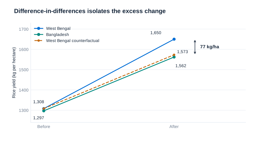
Operation Barga, introduced in West Bengal in 1978, sought to regulate tenancy rents and strengthen sharecroppers' security. Improved security and a greater retained share of output could change effort, investment and bargaining incentives. A familiar illustration associated with Banerjee, Gertler and Ghatak's work compares rice yields in West Bengal with those in neighbouring Bangladesh, which did not receive the same reform. The outcome is measured in kilograms per hectare, so differences retain that unit.

Table 17. Rice yields before and after tenancy reform (kg/ha)
Group	Before reform	After reform	Change
West Bengal	1,308	1,650	342
Bangladesh	1,297	1,562	265
West Bengal minus Bangladesh	11	88	77

The treated group's increase is $1650 - 1308 = 342$ kg/ha. The comparison group's increase is $1562 - 1297 = 265$ kg/ha. Their difference is therefore $342 - 265 = 77$ kg/ha. The same answer follows from $88 - 11$ . Using only the treated group's increase would attribute all 342 kg/ha to the reform. Using only the final group difference would produce 88 kg/ha and ignore the initial gap.

The counterfactual post-reform yield for West Bengal is its initial yield plus the comparison group's increase:

{\hat{Y}}_{T, P o s t} (0) = 1308 + (1562 - 1297) = 1573 .

The estimated effect is the vertical gap between actual yield, 1,650, and counterfactual yield, 1,573: precisely 77 kg/ha. The control group's actual final yield is 1,562, which is not the treated group's counterfactual because their initial levels differed. Relative to the estimated counterfactual, 77 kg/ha is about 4.9%; relative to initial treated yield, it is about 5.9%. These percentages answer different questions and must be labelled accordingly. Four means suffice to compute a point estimate, but do not supply a standard error or establish that the identifying assumptions hold.

West Bengal rises from 1,308 to 1,650 kilograms per hectare and Bangladesh from 1,297 to 1,562. A dashed counterfactual for West Bengal reaches 1,573, leaving a 77-kilogram-per-hectare treatment contrast. — **Figure 14.** Rice yields rise by 342 kg/ha in West Bengal and by 265 kg/ha in Bangladesh. Under parallel untreated trends, the treated counterfactual is 1,573 kg/ha and the difference-in-differences estimate is 77 kg/ha: (1,650 − 1,308) − (1,562 − 1,297).

Parallel trends is a counterfactual assumption

Let $Y_{i t} (0)$ denote the outcome that unit $i$ would have without treatment, and $Y_{i t} (1)$ the outcome under treatment. Let $D_{i} = 1$ indicate membership in the treated group. Parallel trends requires equal average changes in untreated potential outcomes:

E [Y_{i, P o s t} (0) - Y_{i, P r e} (0) ∣ D_{i} = 1] = E [Y_{i, P o s t} (0) - Y_{i, P r e} (0) ∣ D_{i} = 0] .

This does not require equal initial outcome levels. It also does not require observed outcomes to remain parallel after treatment; a treatment effect is exactly what may make observed paths diverge. The assumption concerns the path the treated group would have followed without treatment. That path is unobserved after treatment begins, which is why parallel trends cannot be directly verified from the post-treatment data.

Under no anticipation and an untreated comparison group, the observed DiD equals the average treatment effect on the treated plus the difference in their untreated trends. Parallel trends sets the latter term to zero. This identifies an effect for the treated population, not necessarily the effect that would arise if every other group adopted the same policy. Similar geography or similar baseline means can help justify a comparison, but neither property guarantees similar counterfactual changes.

Anticipation, spillovers and composition

No anticipation means that behaviour before the designated treatment date has not already responded to the impending policy. If a reform is announced in advance and farmers begin investing immediately, treating the announcement-to-implementation period as an unaffected baseline can distort the estimate. The relevant treatment date should reflect when behaviour could change.

No interference across comparison groups requires careful thought about spillovers. A neighbouring region may be attractive as a control because it faces similar conditions, yet trade, migration or policy competition can transmit the treatment into that region. If the comparison group's outcome also responds, the estimated contrast is generally not the treated group's effect relative to a fully untreated world.

Group composition must also remain suitable for the comparison. In repeated cross-sections, different people may be observed before and after, and treatment-induced migration or survey nonresponse can change the population represented by a group mean. A panel reduces some composition concerns but can still suffer selective attrition. Time-varying covariates may improve a conditional comparison when they are appropriate confounders; controlling for a variable caused by the treatment can instead remove part of the effect being estimated or introduce bias.

The two-group, two-period regression

The elementary DiD can be estimated by an interaction regression:

Y_{i t} = β_{0} + β_{1} D_{i} + β_{2} P o s t_{t} + β_{3} (D_{i} \times P o s t_{t}) + u_{i t} .

Here $P o s t_{t} = 1$ after treatment and zero before. The intercept $β_{0}$ is the comparison group's pre-treatment mean. The coefficient $β_{1}$ is the treated group's initial difference from that mean. The coefficient $β_{2}$ is the comparison group's change over time. The interaction $β_{3}$ captures the treated group's additional change. These statements follow by setting the two indicators to zero or one in each of the four cells.

Table 18. Fitted cell means and coefficients in the rice-yield example
Quantity	Regression expression	Value (kg/ha)
Comparison group, before	$β_{0}$	1,297
Treated group, before	$β_{0} + β_{1}$	1,308
Comparison group, after	$β_{0} + β_{2}$	1,562
Treated group, after	$β_{0} + β_{1} + β_{2} + β_{3}$	1,650
Initial group difference	$β_{1}$	11
Comparison-group change	$β_{2}$	265
Additional treated-group change	$β_{3}$	77

The saturated regression reproduces the four sample cell means and the same DiD point estimate. If weights or additional regressors are introduced, the resulting estimate reflects those choices and need not equal the simple unweighted four-mean contrast. A coefficient in kilograms per hectare remains an absolute yield effect; a log-outcome model would instead require interpretation on the log scale and an explicitly justified transformation.

Many units, many periods and treatment intensity

With many units and periods, fixed effects provide a convenient regression representation:

Y_{i t} = α_{i} + λ_{t} + τ D_{i t} + u_{i t} .

Unit effects replace a single average treated-versus-control level difference with an intercept for each unit. Period effects replace a single post indicator with an intercept for each date. The treatment variable $D_{i t}$ records actual exposure in that unit and period. This flexibility is useful, but it does not mean every two-way fixed-effects coefficient automatically estimates a well-defined average causal effect.

Minimum legal drinking-age policies illustrate why treatment need not be binary or start at a common date. Following the end of US Prohibition, states set different age rules; several lowered their thresholds during the early 1970s. In the historical comparison, Alabama lowered its threshold to 19 in 1975, Arkansas retained 21, and Tennessee lowered it to 18 in 1971 before raising it to 19 in 1979. Later federal policy encouraged a minimum age of 21, adopted in every state by 1988. These changes create variation in the fraction of young adults legally able to purchase alcohol.

Define $L E G A L_{s t}$ as the proportion of 18–20-year-olds in state $s$ and year $t$ who are legally eligible. A model for their mortality rate can be written as

Y_{s t} = α_{s} + λ_{t} + τ L E G A L_{s t} + u_{s t} .

When $L E G A L$ is coded between zero and one and $Y$ is deaths per 100,000 people, $τ$ describes the fitted difference associated with moving from none to all of the age group being eligible. A 10-percentage-point increase in eligibility corresponds to $0.10 τ$ . The model imposes a linear relationship in treatment intensity; stronger assumptions are needed to interpret differences across doses causally. State effects absorb fixed state differences and year effects absorb common annual shocks, while simultaneous policy changes or differential mortality trends can still confound the estimate.

Pre-treatment evidence and event studies

Several pre-treatment periods make a research design more informative because they reveal whether the groups were already moving differently. For a common treatment date $t_{0}$ , an event-study specification replaces one post-treatment coefficient with treatment-group interactions for relative dates:

Y_{i t} = α_{i} + λ_{t} + \sum_{k \neq - 1} θ_{k} (D_{i} 𝟏 {t - t_{0} = k}) + u_{i t} .

The period immediately before treatment, $k = - 1$ , is omitted as the reference. Pre-treatment coefficients measure how the treated–comparison gap at earlier dates differs from that reference gap. Post-treatment coefficients describe how the gap evolves after exposure. Plotting point estimates with appropriate uncertainty intervals makes timing, precision and persistence easier to assess than a single average coefficient.

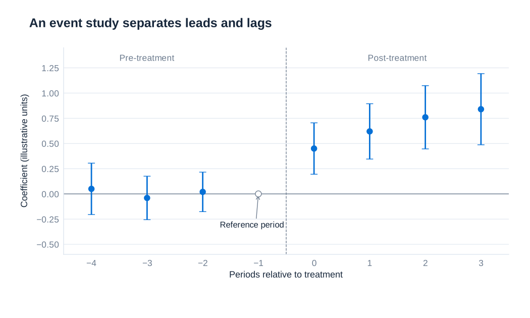
Constructed event-study coefficients are near zero before treatment and positive after treatment. Period minus one is marked as the omitted reference, not an estimated zero coefficient. Error bars are illustrative confidence intervals. — **Figure 15.** An illustrative event study reports coefficients relative to the omitted period −1. Bars are constructed 95% normal-approximation intervals. Near-zero leads do not prove parallel trends: tests may lack power and post-treatment counterfactual trends remain unobserved.

Pre-treatment estimates near zero are consistent with parallel trends, but do not prove the assumption. A test can have low power, confidence intervals can permit economically substantial differences, and a new post-treatment shock may affect the groups differently despite similar histories. Conversely, significant pre-treatment differences may reveal anticipation, an unsuitable comparison group or misspecification. Both individual estimates and a joint test of pre-treatment coefficients are informative, alongside substantive knowledge of the setting. The credibility claim concerns counterfactual post-treatment trends, so a nonsignificant pretrend test must never be presented as conclusive validation.

Differential trends and their limits

A conventional DiD fails when treated and comparison units would have continued along different trends without treatment. One sensitivity specification adds unit-specific linear trends:

Y_{i t} = α_{i} + λ_{t} + θ_{i} t + τ D_{i t} + u_{i t} .

The coefficient $θ_{i}$ permits each unit to have a stable linear deviation from the common time path. The treatment coefficient then reflects departures from those fitted paths. This replaces simple parallel trends with a stronger functional-form claim about how untreated differences would have evolved. It is not a general repair for any arbitrary divergence.

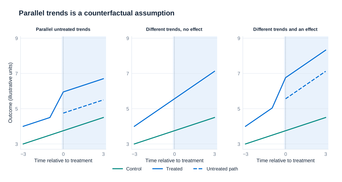
Three schematic time-series panels show parallel trends with a treatment jump, different underlying trends without a treatment jump, and different trends with a jump. Dashed treated lines show the known untreated path in these constructed examples. — **Figure 16.** Three constructed scenarios separate parallel untreated trends, differential trends without treatment, and differential trends plus a treatment effect. In the middle panel a basic two-period DiD would confound the different underlying trends with an effect. Any trend-adjusted analysis adds assumptions about how the untreated trend would continue.

Three cases clarify the distinction. With parallel untreated paths and a discrete treatment-induced jump, a standard DiD can recover the jump. With nonparallel untreated paths and no treatment effect, the changing group gap can produce a spurious DiD. With nonparallel paths plus a genuine jump, a correctly specified differential-trend model may separate the discontinuity from smooth pre-existing divergence. However, if treatment effects emerge gradually, fitting unit-specific trends to all periods can absorb part of the effect. Conclusions should therefore consider how trend estimates, treatment dynamics and the chosen pre-treatment window interact.

Staggered adoption and heterogeneous effects

When units adopt treatment at different dates and effects vary across cohorts or exposure durations, a conventional two-way fixed-effects regression can use already-treated units as controls for newly treated units. The resulting coefficient can combine comparisons with difficult or even negative weights and need not equal the intended average treatment effect on the treated. A clean elementary DiD interpretation should not be carried over automatically.

Modern approaches estimate effects for treatment cohorts and dates using suitable never-treated or not-yet-treated comparison units, then aggregate those effects transparently. The researcher must define the target population and weighting scheme, justify parallel trends and no anticipation for the selected comparisons, and identify which post-treatment horizons have credible controls. Reversible policies and continuous treatment require additional care because methods designed for a single absorbing adoption date do not automatically apply.

Uncertainty and the effective amount of information

Outcomes and policy exposures often persist over time. Treating every person-year or state-year as independent can make standard errors much too small. In a state-policy design, clustering by state allows disturbances to be correlated across years and across observations sharing that state. If important shocks cross state boundaries, state clustering alone may not capture the entire dependence structure. The appropriate level follows the research design and the plausible correlation of the disturbances.

More observations inside the same few policy units do not create many independent policy experiments. The relevant issue is the number and balance of independent clusters, especially the number receiving treatment. There is no universal threshold at which cluster-robust inference becomes automatically reliable. With few clusters, methods such as suitable small-sample corrections, wild-cluster bootstrap procedures or design-based randomization inference may be needed, with assumptions explained. The four aggregate rice-yield means, for example, cannot alone justify a conventional standard error. A complete DiD study combines transparent arithmetic, a defensible counterfactual and an uncertainty calculation matched to the actual assignment structure.

Torna all’inizio ↑

Ripetizioni personalizzate · Da 15€/h

Un dubbio da chiarire?
Studiamolo insieme.

Offro lezioni personalizzate per studenti delle superiori e dell’università: spiegazioni chiare, esercizi guidati e un metodo costruito sulle tue esigenze. Scopri le materie e le tariffe, oppure prenota una lezione per lavorare sul tuo programma.

Prenota una lezione Scopri il tutoraggio