
3. Omitted Variable Bias and Measurement Error
A regression coefficient is useful only when its interpretation matches the process that produced the data. A large sample can make an estimate very precise while leaving it systematically wrong about the relationship of interest. Two particularly important threats are omitted variables, which place relevant determinants of the outcome inside the regression error, and measurement error, which separates the variables recorded in a dataset from the economic quantities they are supposed to represent. Understanding these problems requires distinguishing uncertainty around an estimate from bias in its target.
Consistency, exogeneity, and the target of estimation
Consider the population relationship . The parameter describes the relationship we seek to estimate; the error collects determinants of the outcome that are outside the model. In a simple regression with an intercept, the OLS slope can be expressed as a sample covariance divided by a sample variance. Under a law of large numbers and a positive, finite variance of , its probability limit is
The equation identifies the central consistency requirement: the regressor must be uncorrelated with the error for OLS to converge to this structural slope. The stronger condition also supports the usual conditional interpretation and, with suitable sampling assumptions, finite-sample unbiasedness. Consistency means that the estimator approaches the target as the sample grows; unbiasedness concerns the estimator's expectation at a particular sample size. Neither property is established simply by obtaining a small standard error.
The statement that OLS is the best linear unbiased estimator additionally requires the assumptions of the Gauss–Markov theorem, including the appropriate homoskedastic and uncorrelated error structure. Those efficiency assumptions should not be confused with the exogeneity conditions needed to recover the target coefficient. A regression can have heteroskedastic errors and still estimate the slope consistently, whereas an omitted confounder can make the coefficient inconsistent even with perfectly homoskedastic errors. If the goal is only a best linear prediction, OLS can estimate that predictive projection without identifying a causal effect.
Deriving omitted variable bias
Suppose that the relevant population model contains an additional variable :
where is uncorrelated with and . If is omitted, the error in the shorter regression becomes . The omission matters for the coefficient on when two conditions hold together: helps determine , so that , and is correlated with . Correlation with alone is insufficient if the omitted variable has no effect on the outcome in the relevant population relationship.
Write the population linear projection of the omitted variable on the included regressor as
This projection is an algebraic description of association; it does not require to cause . Substitution gives
The short-regression slope therefore converges to a combination of the direct slope and the association operating through the omitted variable:
This is a statement about the probability limit, not an exact decomposition of every realized estimate: an individual sample also contains sampling variation. In multiple regression, the corresponding omitted-variable relationship is conditional on the controls already included. What matters is whether the omitted variable remains related to the regressor after those controls have been taken into account.
Determining the direction of the bias
The sign of the bias is the product of two signs. First ask whether an increase in the omitted variable raises or lowers the outcome, holding the included regressor fixed. Then ask whether observations with larger values of the included regressor tend to have larger or smaller values of the omitted variable. Keeping these two questions separate prevents an intuitive story from being substituted for an actual sign calculation.
| Effect of omitted variable on the outcome | Association with the included regressor | Bias in the short-regression slope |
|---|---|---|
| Positive: | Positive: | Positive: slope is shifted upward |
| Positive: | Negative: | Negative: slope is shifted downward |
| Negative: | Positive: | Negative: slope is shifted downward |
| Negative: | Negative: | Positive: slope is shifted upward |
“Upward” means numerically larger, and “downward” means numerically smaller. Neither expression is synonymous with “closer to zero.” A negative bias makes a positive coefficient smaller, but makes a negative coefficient more negative; sufficiently strong confounding can even reverse its sign. When several relevant variables are omitted, their contributions can reinforce or offset one another, so identifying one plausible confounder need not identify the sign of the total bias.
Test scores, class size, and family income
A school-district example relates average test scores to the student-to-teacher ratio. A higher ratio means more students per teacher, so the coefficient is measured in test-score points per additional student per teacher. The unadjusted regression gives an intercept of approximately and a slope of approximately . It predicts that districts differing by one student per teacher differ by about 2.28 test-score points on average. This is initially an association between districts, not an identified effect of hiring teachers.
Family income offers a plausible explanation for part of that association. Suppose that higher family income raises achievement through resources and opportunities, so , and that richer districts tend to have lower student-to-teacher ratios, so . Their product is negative. The short regression then attributes some of the achievement advantage associated with income to the lower ratio, making the estimated ratio coefficient more negative than the coefficient obtained with a suitable income control.
In the illustrated comparison, the displayed ratio slope changes from approximately without income to with income. A five-unit increase in the ratio is consequently associated with about points using the first displayed slope and points using the adjusted slope. These are calculations from the reported regression slopes, not experimental policy effects. The upward movement of the coefficient is consistent with the predicted direction of omitted income bias, but does not establish that all confounding has disappeared.

The adjustment should be understood as comparing districts after accounting for the modeled income relationship. Other determinants, including family background, school composition, and the way resources are allocated, may remain relevant. A fitted intercept near 699 is also an extrapolation to a ratio of zero, outside the useful comparison range; it should not be interpreted as the score a real district would obtain with no students per teacher.
Addressing omitted variables without adding bad controls
The most direct response is to collect and include a well-measured confounder. This works only if the expanded model provides an adequate representation of the relevant conditional relationship and sufficient variation remains to estimate the effect. Controlling for a variable does not automatically remove every dimension of selection associated with it. For example, one income measure may leave substantial differences in family resources unexplained, and a purely linear adjustment may be inadequate for a strongly nonlinear relationship.
A proxy can help when the confounder itself is unavailable, but an imperfect proxy generally leaves residual confounding. Instrumental variables can address certain endogeneity problems when an instrument is relevant for the endogenous regressor and satisfies a credible exclusion restriction and exogeneity condition. Panel methods can remove unobserved characteristics that remain constant within a unit over time. Each approach replaces one identification challenge with explicit assumptions that must be defended; none is a mechanical guarantee of a causal coefficient.
Control selection should follow the causal question. A variable caused by the treatment can be a mediator rather than a pre-existing confounder. Adjusting for it may remove part of the total effect that the researcher wants to estimate. Conditioning on a common consequence of treatment and unobserved outcome determinants can also create bias. A thoughtful specification therefore begins with a description of the economic process and the timing of variables, rather than with a search for the largest possible collection of controls.
Measurement error in an explanatory variable
Economic variables are frequently measured imperfectly. National output relies on incomplete records and estimation; time-use surveys depend on recall; undocumented migration is difficult to count; self-reported income and happiness may be recorded inaccurately. Measurement error can reflect random noise, systematic reporting behavior, or a mismatch between a recorded indicator and the underlying concept.
Let denote the true regressor and let the observed value be . Suppose the population model is . In the classical additive case, assume , , , and . Substituting into the model yields
The minus sign is essential. The observed regressor contains the measurement error positively, while the new regression disturbance contains it multiplied by . Consequently,
Thus even error that is unrelated to the true regressor creates correlation between the observed regressor and the composite regression disturbance. Calling the measurement error “random” does not make the resulting regression exogenous.
Attenuation, reliability, and nonclassical error
The classical assumptions imply and . The probability limit of the observed-regressor slope is therefore
The reliability ratio lies between zero and one when true variation is positive and measurement-error variance is finite. It equals one when there is no measurement error. As noise becomes more important relative to true variation, the slope is pulled further toward zero. A positive true coefficient is attenuated downward; a negative true coefficient is attenuated upward. Attenuation is therefore a reduction in magnitude, not an invariably downward numerical bias.
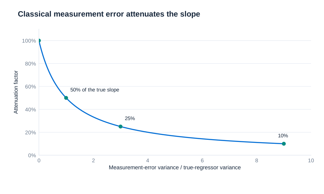
For a hypothetical example, if true variation and measurement-error variation are equal, then : a true slope of 4 is estimated near 2 in a sufficiently large sample, while a true slope of is estimated near . More observations concentrate the estimator around this attenuated target; they do not remove the distortion. Better measurement, validation information, or a suitably valid instrument can help identify the desired coefficient.
Nonclassical error violates one or more of the classical restrictions. High-income respondents might underreport income more strongly, or reporting quality might depend on the outcome. The bias can then have either sign. Even classical error in one variable of a multiple regression need not move every estimated coefficient toward zero: correlations among regressors can transmit the problem to other coefficients. The simple reliability formula should therefore be used only for the model and assumptions under which it was derived.
Measurement error in the outcome and practical interpretation
Now suppose the true outcome satisfies , but the observed outcome is . The estimated relationship becomes
If the original error is exogenous and the outcome measurement error has conditional mean zero given , the composite error remains exogenous. The slope can therefore remain consistent. If is also uncorrelated with , its variance adds to the original disturbance variance, generally reducing precision. Under those restrictions, classical outcome noise increases uncertainty without producing the regressor attenuation described above.
This conclusion is conditional, not universal. If people with higher systematically overreport the outcome, then varies with and the slope can be biased. Correlation between measurement error and the original disturbance also changes the simple variance-addition result. A careful empirical analysis identifies what is measured, how it is recorded, and why the proposed error assumptions are plausible. The central distinction is whether the problem changes the coefficient's target, its precision, or both.