
4. Hypothesis Testing and Statistical Inference
A point estimate is one realization of a procedure applied to data. Another sample could produce another estimate, even if the population relationship remained unchanged. Statistical inference measures this sampling uncertainty and uses it to assess hypotheses and construct confidence intervals. Its conclusions depend both on a credible model for the coefficient and on a credible estimate of the coefficient's variability. Neither a small p-value nor a narrow interval repairs omitted variable bias or an invalid causal design.
Random sampling and random assignment answer different questions
Random sampling concerns how observations enter a dataset. A simple random sample supports inference from the observed units to the population from which they were drawn. Random assignment concerns how treatment is allocated among units and can make treatment status independent of their potential outcomes. A study can have random assignment without drawing a representative population sample, or a representative sample without random treatment assignment.
The distinction separates identification from generalization. Random assignment can provide a credible treatment comparison within the studied group; extending that effect to other groups may require additional assumptions. Conversely, randomly sampling people does not make their education, income, or treatment choices exogenous. In observational regression, uncertainty about which units were sampled and bias from how the regressor is related to unobserved determinants are different problems.
The sampling distribution describes the estimates that would arise if the sampling procedure were repeated under the same population and model. This is a conceptual repetition, not a claim that the researcher actually observes many populations. Standard errors approximate the spread of that distribution using the available data and assumptions about dependence. If the sampling process involves households, schools, regions, or repeated observations, the relevant independent units may be groups rather than individual rows.
Standard errors measure uncertainty in an estimator
The standard deviation of an outcome describes variation across observations. The standard error of an estimator describes variation across hypothetical repeated estimates. These quantities answer different questions and have different units. A regression slope's standard error is measured in the same units as that slope: for a test-score regression on students per teacher, it is test-score points per unit of the ratio.
For a simple regression with an intercept, conditionally homoskedastic and uncorrelated errors, and a valid conditional-mean specification, the slope variance conditional on the observed regressors is
Because the disturbance variance is unknown, it is estimated from residuals. With two estimated coefficients, the usual estimator is . The conventional slope standard error is the square root of the estimated coefficient variance. The corresponding large-sample intuition is .
More unexplained outcome variation increases uncertainty; more independent observations and more useful regressor variation reduce it. In multiple regression, the useful variation in a regressor is what remains after accounting for the other regressors. Strong collinearity can therefore produce large standard errors even in a dataset with many observations. These relationships concern precision under the model, not whether the model identifies a causal effect.
Null hypotheses, t-statistics, and reference distributions
A null hypothesis specifies a value for a population parameter, such as . For a two-sided alternative, , the t-statistic measures the estimated distance from the null in standard-error units:
When , this reduces to the familiar coefficient-to-standard-error ratio. A value of means that the estimate is four estimated standard errors below the hypothesized value. It is the population coefficient that the hypothesis concerns; the observed estimate is already known and is not itself a random unknown after the data have been observed.
Under normally distributed, conditionally homoskedastic independent errors and the usual linear model assumptions, the conventional t-statistic has an exact Student t distribution with degrees of freedom, where includes the intercept. With heteroskedasticity-robust standard errors, that exact finite-sample result generally does not apply. Under appropriate regularity conditions, the studentized statistic instead approaches a standard normal distribution as the effective sample size grows. Software may use a t reference distribution with a degrees-of-freedom adjustment as an approximation; its validity should be assessed in light of the design.
The central limit theorem applies to standardized averages
The central limit theorem explains why normal approximations can be useful even when individual observations are not normally distributed. For independent and identically distributed random variables with mean and finite positive variance , the basic theorem states
The raw observations do not become normal as the sample grows. The centered and scaled sample mean approaches a normal distribution, while the unscaled sample mean becomes concentrated near its population mean. Regression inference uses a related argument because, under suitable assumptions, an estimator's error can be represented approximately as an average of random contributions. Valid studentization additionally requires a consistent standard-error estimate.
Consider a Bernoulli variable that equals one with probability 0.8 and zero otherwise. Each observation remains binary for every sample size. Its mean is 0.8 and its variance is . The standard deviation of its sample mean is therefore . At sample sizes 10, 100, 1,000, and 10,000, this becomes approximately 0.1265, 0.0400, 0.01265, and 0.0040 respectively.
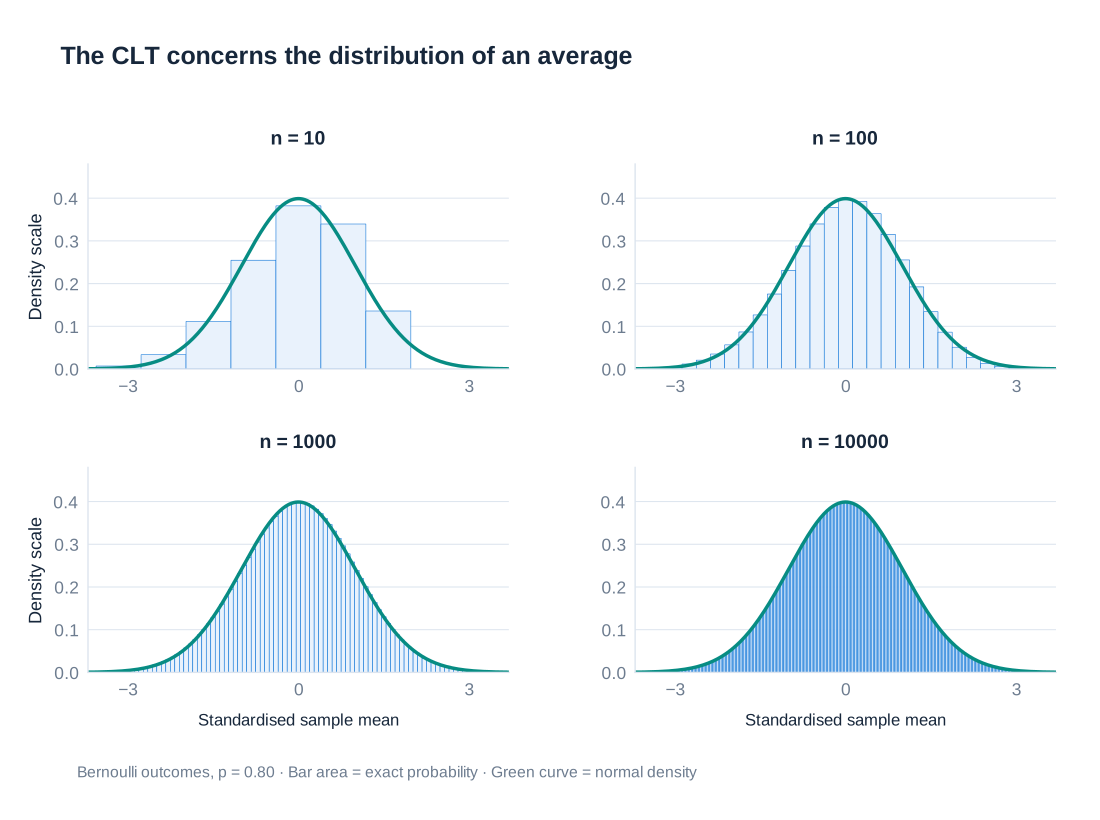
The distribution of the sample mean is discrete, with possible values separated by . At small sample sizes it can be visibly asymmetric because the success probability is high; at larger sizes its standardized shape is well approximated by the normal distribution. The approximation is not an automatic consequence of a large row count. Heavy tails, dependence, weak identification, or only a few independent clusters can undermine the conditions required for familiar large-sample reasoning.
Rejection regions and statistical significance
A significance level specifies the probability of rejecting a true null hypothesis that the testing procedure is designed to control under its assumptions. For a two-sided test using a standard normal reference distribution, a 5% significance level places 2.5% in each tail and uses critical values approximately and . Rejecting when therefore identifies estimates unusually far from the null relative to their estimated sampling variability.
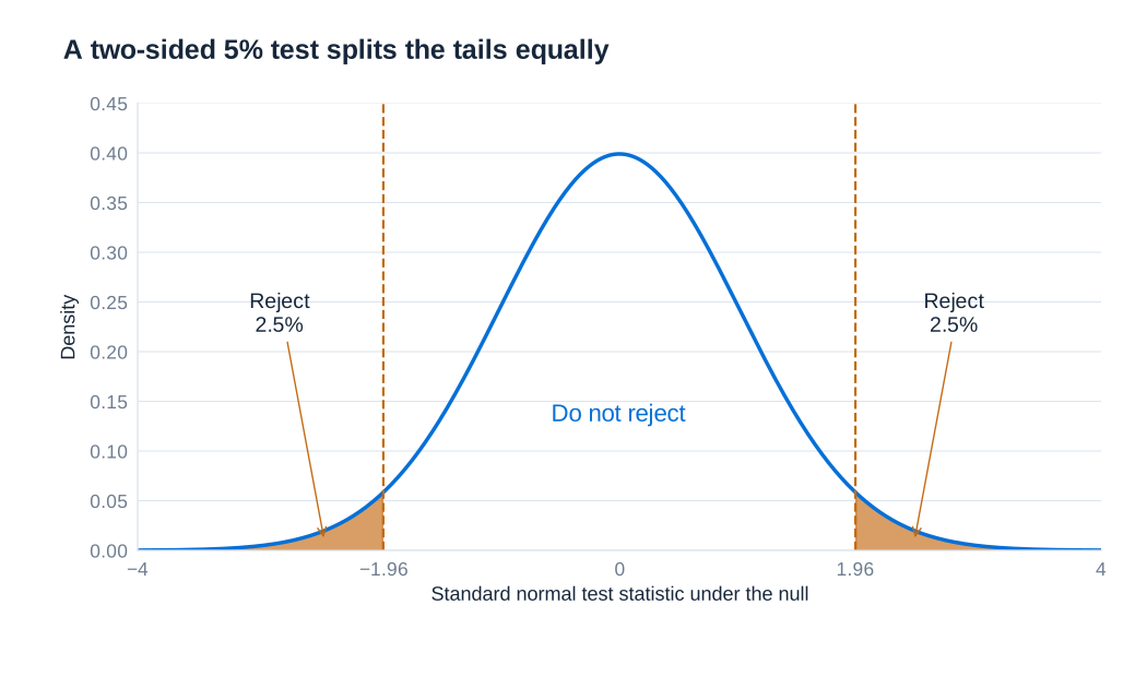
The familiar statement that about 95% of a normal distribution lies within two standard deviations is a useful approximation; the exact central normal probability between and is about 95%, whereas the interval from to contains about 95.45%. An exact t test uses a critical value based on its degrees of freedom, which is larger than 1.96 in finite samples.
A rejection does not establish a 95% probability that the alternative is true. A failure to reject does not establish that the null is true. Tests can make a Type I error by rejecting a true null or a Type II error by failing to reject a false null. Power is the probability of rejecting under a specified alternative; small samples and noisy measurements can make economically important effects difficult to detect. One-sided tests allocate their rejection region to one direction and should be justified before examining the estimated sign.
P-values express incompatibility with the null model
A p-value is the probability, calculated under the null hypothesis and the maintained statistical assumptions, of obtaining a test statistic at least as extreme as the observed one. For a two-sided standard normal test,
where is the standard normal cumulative distribution function. With an appropriate t reference distribution, its cumulative distribution replaces . The calculation includes outcomes more extreme than the observed statistic; it is not the probability of obtaining exactly that estimate.
A p-value of 0.04 means that, if the null and the statistical model held, a statistic at least as extreme would occur with probability 4%. It is evidence against that null at the 5% level, not a 4% probability that the null is true or proof that the estimated effect is causal. A p-value of 0.50 indicates weaker evidence against the null, but does not demonstrate that the true effect is zero. It may reflect a small effect, imprecise estimation, or both.
Statistical significance also differs from economic importance. A tiny effect can yield a small p-value in a very large sample, while a large but imprecise estimate may not cross a conventional threshold. The effect's units, confidence interval, substantive relevance, and identification assumptions should accompany the p-value. Testing many outcomes or specifications and reporting only the smallest p-values changes the interpretation of nominal significance levels.
Confidence intervals retain information about magnitude
A two-sided confidence interval combines the estimate with a margin of uncertainty:
where is the critical value corresponding to the confidence level and reference distribution. A 95% confidence procedure is constructed so that, over repeated samples under its assumptions, approximately 95% of the resulting intervals contain the fixed population parameter. Once a particular interval has been calculated, its endpoints are fixed and the parameter either lies inside it or does not; the frequentist interpretation is not a posterior probability assigned to that parameter.
When the interval and test use the same assumptions and reference distribution, the interval contains the null parameter values that the corresponding two-sided 5% test would not reject. If zero is outside a 95% interval, the coefficient is statistically distinguishable from zero at that level. If zero is inside, the interval may still include economically substantial positive or negative values. Reading the whole interval therefore gives more information than attaching a significance star to the point estimate.
A complete test-score regression example
The regression of district average test scores on the student-to-teacher ratio uses 420 observations and heteroskedasticity-robust standard errors. The estimated equation is . The regression explains about 5.12% of the sample outcome variation, so . Its root mean squared error is 18.581 test-score points. These fit statistics describe the regression's sample fit and residual scale, not the validity of a causal interpretation.
| Regressor | Coefficient | Robust standard error | t-statistic | Two-sided p-value | 95% confidence interval |
|---|---|---|---|---|---|
| Student-to-teacher ratio | −2.279808 | 0.5194892 | −4.39 | < 0.001 | [−3.300945, −1.258671] |
| Intercept | 698.933 | 10.36436 | 67.44 | < 0.001 | [678.5602, 719.3057] |
Testing a zero ratio coefficient gives . The output uses 418 residual degrees of freedom and reports for the one-coefficient restriction; in this case the F-statistic is the squared t-statistic, up to rounding. The two-sided p-value for the ratio coefficient using this t reference is approximately 0.0000145. A displayed p-value rounded to 0.000 therefore means very small, not literally zero.
The 95% t critical value for 418 degrees of freedom is approximately 1.96566. Applying it gives the reported interval . The normal approximation using 1.96 gives the very similar interval . Mixing a heavily rounded coefficient, a different critical value, and more precise printed endpoints would create apparent arithmetic discrepancies, so calculations should retain the original precision until the final reporting step.
The interval describes uncertainty about the regression association under the maintained model. A one-unit higher ratio is associated with a decrease between about 1.26 and 3.30 test-score points at this confidence level. The omitted-income argument in the preceding chapter still applies: robust standard errors address a variance problem, not the confounding that can separate this coefficient from the causal effect of changing class size.
Heteroskedasticity and robust standard errors
Homoskedasticity means that the conditional disturbance variance is constant: . Heteroskedasticity means that this variance changes with the regressors or other observed characteristics. A graph may show observations spreading more widely around the conditional mean at larger values of . The slope of that mean and the width of the disturbance distribution are separate features of the model.
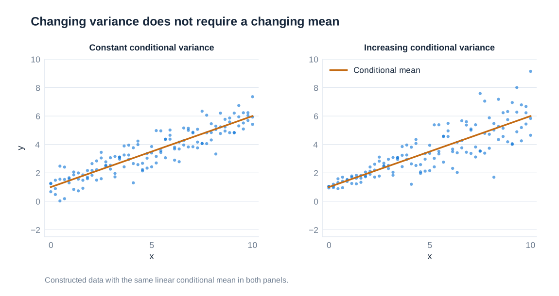
If exogeneity and the relevant sampling conditions continue to hold, heteroskedasticity does not by itself make OLS coefficients inconsistent. It does invalidate the conventional homoskedastic variance formula. Standard errors calculated from that formula can be too small or too large; downward distortion and overstated significance are common concerns, but the direction is not guaranteed.
For simple regression with an intercept and independent observations, the basic heteroskedasticity-robust variance estimator can be written
Each squared residual contributes separately, allowing the disturbance variance to differ across observations. Other robust estimators adjust for degrees of freedom or leverage; the HC1 version multiplies the variance estimate by . Changing from conventional to robust standard errors leaves the OLS point estimates unchanged when the regression sample and specification are unchanged, but can change confidence intervals, t-statistics, and p-values.
Heteroskedasticity-robust standard errors are not a general correction for dependence between observations, omitted variables, or measurement error. They can also be unreliable in small samples or with influential observations. The word “robust” describes the particular variance restriction relaxed, not immunity from all modeling problems.
Dependent observations and clustered inference
Observations within a group often share unobserved shocks. For repeated state observations, a simple example is , where is a persistent state component. Two observations on the same state can then have correlated errors across time. Alternatively, represents a common year shock affecting different states. The indices matter because these processes imply different dependence patterns and potentially different clustering choices.
Federal aid received by a state in successive years, for example, can be affected by persistent state characteristics and ongoing programs. Treating each state-year as an independent source of information can exaggerate precision. Ordinary heteroskedasticity-robust standard errors allow different individual variances but omit the covariance terms between different observations. Cluster-robust standard errors retain those within-group covariance terms while relying on suitable independence or weak dependence across clusters.
Writing the design matrix for cluster as and its residual vector as , the basic cluster-robust covariance estimator is
Finite-sample corrections are often applied in practice. Clustering does not require averaging the data into one observation per group: the regression may keep all individual observations while the variance calculation recognizes their dependence. The appropriate level follows the design, treatment assignment, and plausible shared shocks. With persistent state dependence, state clustering allows arbitrary within-state correlation over time. Dependence arising both within states and across states in the same year may require a method that accommodates both dimensions.
Conventional clustered inference relies primarily on the number and behavior of independent clusters, not simply the total number of rows. There is no universal cutoff at which it becomes reliable: a few very large clusters, uneven treatment allocation, or high leverage can remain problematic even when a numerical rule of thumb is met. With few clusters, appropriate small-sample methods or design-based inference may be needed. Finally, serial dependence must not be confused with exogeneity: changing the standard-error estimator does not repair a coefficient made inconsistent by correlation between regressors and disturbances.