
5. Nonlinear Relationships and Functional Forms
Why a straight line may be too restrictive
A linear regression assigns a constant slope to a regressor: in , increasing by one unit changes the fitted outcome by , wherever the change begins. That can be a useful local approximation, but it is not a universal description of economic behaviour. An additional hour of study may improve performance more when a student has studied little than after prolonged preparation. Additional police officers may have different associations with crime in understaffed and heavily staffed cities. The association between household income and educational performance may also flatten as income rises. Each example motivates examining the shape of the relationship rather than imposing a constant slope automatically.
A scatterplot of average district income and average test scores can help reveal this issue. If the fitted straight line systematically misses the curvature of the cloud, its residuals may be positive in some income ranges and negative in others. A nonlinear specification can represent that pattern more accurately. This is a statement about conditional means, not a guarantee of causation: income may be correlated with family resources, parental education, neighbourhood conditions and other determinants of achievement. Changing the curve does not eliminate omitted-variable bias.
“Nonlinear” can refer to different things. A quadratic regression is nonlinear in the regressor but linear in its unknown coefficients. Ordinary least squares can therefore estimate it after creating the squared regressor. A model such as remains a linear regression model in this statistical sense. By contrast, a probability model with a normal cumulative distribution function is nonlinear in its coefficients and generally requires a different estimation method.
Quadratic specifications and changing marginal effects
A quadratic specification extends the straight line by adding a squared term. For district income and average test score , write:
The coefficient on is no longer the slope everywhere. Differentiating the conditional mean gives the marginal effect, measured in score points per income unit:
If , the slope decreases with income, producing a concave curve; if , the slope increases. The curve turns where , provided . A turning point outside the observed range should not be presented as an empirical discovery. A concave curve estimated over a moderate range may eventually imply falling test scores at implausibly high incomes simply because a polynomial is being extrapolated beyond the data.
The derivative describes an infinitesimal change. For a finite change , the exact fitted difference is . With a one-unit increase, this equals , not just the derivative at the starting point. Distinguishing derivatives from finite differences matters when the interval is large or curvature is strong. It also matters when changing units: measuring income in thousands rather than individual currency units changes both coefficients, although correctly calculated predictions remain the same.
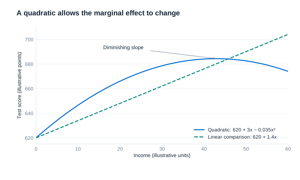
A quadratic should usually include both the linear and squared terms. Dropping the linear term imposes a zero slope at , an assumption that needs an economic justification. Centering income around a meaningful value can make the intercept and linear coefficient easier to interpret without changing fitted values, provided the corresponding transformed model includes all required terms.
Logarithms, proportional changes and skewness
The natural logarithm transforms multiplicative differences into additive differences. Its defining comparison is . Doubling a positive variable always increases its logarithm by , whether the original change is from 1 to 2 or from 100 to 200. This makes logs useful when proportional differences are more informative than absolute differences. Unless another base is explicitly stated, and here denote the natural logarithm, with base .
For a small proportional change , . Increasing income from 100 to 101 is a 1% increase and changes log income by approximately 0.01. Increasing it from 1 to 2 is a 100% increase and changes log income by approximately 0.693; treating this log difference as 1 would be a poor approximation. A log scale does not literally replace every difference by its percentage change. It expresses ratios in logarithmic units, which closely approximate proportional changes only when those changes are small.
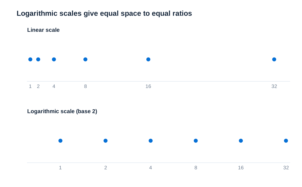
Logging a positive variable also compresses large values. Income often has a long right tail, and a histogram of log income may be more balanced than a histogram of income. However, logging does not guarantee normality, and normally distributed regressors are not an OLS requirement. The transformation should reflect the relationship being modelled and the interpretation required. It also changes the treatment of the data: the real-valued logarithm is undefined at zero and for negative observations. Adding an arbitrary constant before logging changes the model and must not be treated as an innocuous repair.
The linear–log model: outcome units for proportional input changes
When the outcome remains in levels but the regressor is logged, the model is:
The marginal effect in original units is , so an equal absolute increase in has a smaller fitted effect at higher starting values. A 1% increase in changes the fitted outcome by exactly , approximately units of . If is a test score and , a 1% income increase corresponds to approximately 0.2 score points, not a 20% increase in scores. The coefficient remains tied to the units of the outcome.
For any finite comparison from to , the fitted difference is . Doubling the regressor changes the fitted outcome by , not by . The latter would correspond to multiplying the regressor by . Changing the currency unit of a positive income regressor shifts its logarithm by a constant and changes the intercept, while leaving the slope and fitted differences unchanged.
This form is particularly useful when the raw relationship bends but the relationship between the outcome and log input appears closer to a straight line. It embodies a specific shape: with a positive coefficient, the outcome rises at a decreasing rate as the input increases. It cannot represent every possible pattern, such as a genuine U-shaped relationship, without additional terms.
Logged outcomes: semi-elasticities and elasticities
In a log–linear model, , a one-unit increase in changes the fitted log outcome by . The familiar interpretation, an approximately % change in , is accurate only for small coefficients. The exact proportional comparison implied by the fitted log values is:
for a change of units in . Thus a coefficient of 0.04 corresponds to about 4.08% for a one-unit increase, whereas a coefficient of 0.42 corresponds to about 52.20%, making the linear approximation much less satisfactory. A negative coefficient of −0.50 implies about 39.35% lower, not 50% lower.
Strictly, exponentiating a conditional mean of log outcomes describes a conditional geometric mean, not automatically the arithmetic conditional mean of the original outcome. From , the latter is . If the second factor differs across the observations being compared, exponentiating the fitted log difference alone does not give the arithmetic-mean ratio. This distinction matters when predicting expenditure totals or average earnings in currency units.
When both variables are logged, , the slope is an elasticity: . A small 1% increase in corresponds to an approximately % change in . For a finite proportional increase , the exact fitted proportional change is %. The log–log specification assumes a constant elasticity, whereas the log–linear specification assumes a constant semi-elasticity. These are substantive restrictions, not interchangeable ways of presenting the same regression.
Choosing a functional form
Model choice begins with the economic question, the units of measurement and the range of the observations. Scatterplots help identify curvature and influential observations; residual plots help reveal systematic patterns left unexplained by a fitted model. A skewed regressor may motivate considering a log transformation, but skewness alone does not establish that the conditional mean is linear in its logarithm. The same distinction applies to a skewed outcome: logging it changes the estimand and the weight given to proportional versus absolute errors.
Compare candidate models using the same observations when possible, check whether their implications are plausible within the data range, and consider predictive performance on observations not used for estimation. Ordinary values from a level-outcome regression and a log-outcome regression are not directly comparable measures of fit to the same dependent variable. A higher value after changing the outcome scale does not by itself establish a better model.
Interpretability is also valuable. A parsimonious specification that answers a clear question may be more useful than an elaborate curve with unstable behaviour. Report the marginal effects or fitted comparisons actually relevant to the application. In a quadratic model, give the income level at which a slope is evaluated; in a log model, distinguish a one-unit change from a 1% change. An attractive functional form still requires a credible identification strategy before its coefficients receive a causal interpretation.
Interactions and heterogeneous relationships
An additive model, , makes the slope with respect to one regressor independent of the other. That may be too restrictive. Rainfall may have a different association with traffic accidents when impaired driving is more common. Local economic conditions may alter the relationship between a governing party’s policy preferences and public spending. An interaction allows the slope to vary systematically:
The main coefficient is now the slope of when , while is the slope of when . The interaction coefficient measures how one slope changes as the other regressor increases. It should not be interpreted separately as the entire effect of either variable. Retaining both main effects generally avoids imposing arbitrary zero restrictions.
If is a binary indicator, compare predictions at and rather than imagining an infinitesimal change in group membership. In , the group difference is . Its uncertainty depends on both coefficient variances and their covariance:
Consequently, a confidence band for the combined effect cannot be reconstructed from the two reported standard errors alone. Interactions reveal heterogeneity in a fitted relationship; they do not themselves establish why that heterogeneity arises.
Worked example: education, experience and the gender wage gap
Consider a sample of 1,084 individuals from the US Current Population Survey. The outcome is the natural logarithm of hourly wage; education and experience are measured in years; equals 1 for women and 0 for men. Four nested regressions show how interpretation changes as controls and an interaction are added. The numbers in parentheses are standard errors. “Not included” means the regressor is absent from that specification, rather than that its coefficient was estimated as zero.
| Regressor | Model 1 | Model 2 | Model 3 | Model 4 |
|---|---|---|---|---|
| Education, years | 0.0692 (0.00556) | 0.0712 (0.00538) | 0.0874 (0.00562) | 0.0793 (0.00630) |
| Female indicator | Not included | −0.272 (0.0302) | −0.269 (0.0284) | −0.594 (0.147) |
| Experience, years | Not included | Not included | 0.0339 (0.00392) | 0.0347 (0.00391) |
| Experience squared | Not included | Not included | −0.000473 (0.0000847) | −0.000492 (0.0000843) |
| Female × education | Not included | Not included | Not included | 0.0253 (0.0116) |
| Observations | 1,084 | 1,084 | 1,084 | 1,084 |
Model 1 associates an additional year of education with approximately 6.92% higher hourly wages. Adding the female indicator in Model 2 changes that slope and introduces a conditional group comparison. Model 3 adds experience and its square. The positive experience coefficient and negative squared coefficient describe a concave experience profile: early additional experience has a larger fitted association than later additional experience. These changes illustrate why a coefficient is conditional on the rest of the specification; they do not identify which regression has solved all selection problems.
Model 4 allows the education slope to differ by gender. For men, the log-wage slope is 0.0793; for women it is . The exact fitted one-year proportional changes are approximately 8.25% and 11.03%, respectively, under the logged-outcome interpretation described above. The experience slope is . Its fitted turning point is about 35.26 years, whose substantive relevance depends on the observed support and the adequacy of the quadratic specification.
Interpreting and plotting the complete gender contrast
In Model 4, the female coefficient is not the wage gap for every education level. Holding experience constant, the fitted female-minus-male contrast in log wages at education level is:
At zero years of education, this implies a fitted geometric-mean wage ratio of , or about 44.79% lower, rather than 59.4% lower. Zero education may also lie far from most observations, making the intercept contrast a poor headline summary. At 12 years the fitted gap is approximately −25.20%; at 16 years it is −17.24%; and at 18 years it is −12.94%. These percentages use , not the large-coefficient approximation.
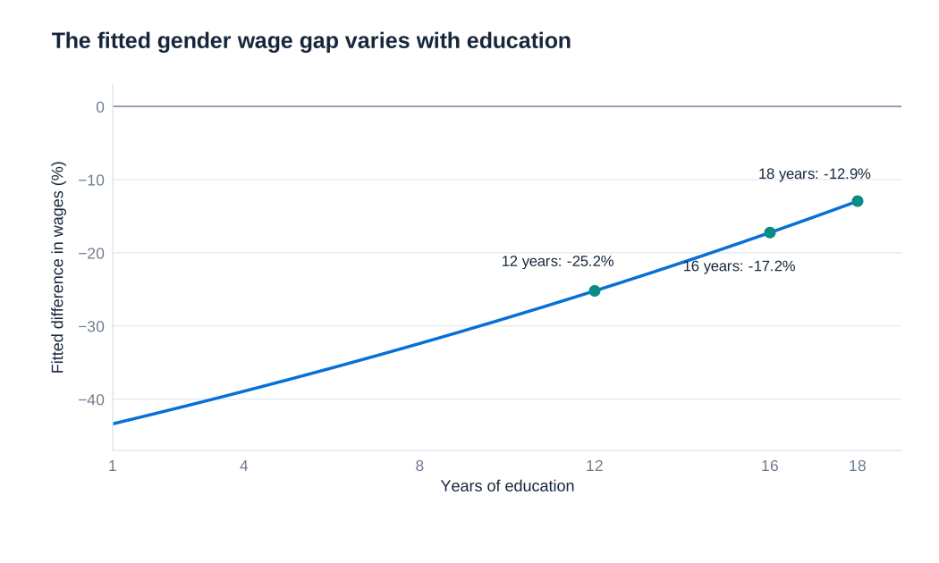
Each additional year of education raises the female-minus-male log-wage contrast by 0.0253. It does not close the exact percentage wage gap by a constant 2.53 percentage points, because exponentiation is nonlinear. Solving the fitted log contrast for zero gives about 23.48 years of education. That algebraic crossing extends beyond the 1–18-year range illustrated here and should not be interpreted as evidence that a particular amount of education eliminates wage inequality.
The regression documents conditional associations. Differences in occupation, hours, job tenure, employment selection and other unobserved characteristics can still affect the estimates. Nor does controlling for such variables automatically settle a discrimination question, since some controls may themselves reflect unequal opportunities. A useful empirical conclusion states precisely which wage measure, sample, controls and education level are being compared, and separates that comparison from any broader causal claim.