
2. Randomisation and linear regression
A causal comparison should isolate the change of interest while holding relevant alternatives constant. Random assignment supplies a benchmark for this task. Linear regression provides a way to describe relationships and, under additional assumptions, to make comparable comparisons using observational data. Understanding the distinction between what an estimator calculates and what its identifying assumptions justify is essential to both approaches.
Health insurance and the problem of comparability
Consider whether health insurance improves health. Comparing insured and uninsured people appears straightforward: calculate average health in each group and subtract. The difficulty is that insurance coverage is not generally assigned at random. People with different coverage can also differ in income, education, employment, age and initial health. These factors may influence both coverage and subsequent outcomes.
The 2009 National Health Interview Survey illustrates the problem. Among married respondents in the reported sample, insured husbands had an average health index of 4.01, compared with 3.70 for uninsured husbands. The reported difference was 0.31. Insured wives also had a higher average index. Yet insured respondents were substantially more educated and had much higher family incomes. The comparison therefore combines insurance with other differences that might matter for health.
| Characteristic | Insured husbands | Uninsured husbands | Difference, husbands | Insured wives | Uninsured wives | Difference, wives |
|---|---|---|---|---|---|---|
| Health index | 4.01 [0.93] | 3.70 [1.01] | 0.31 (0.03) | 4.02 [0.92] | 3.62 [1.01] | 0.39 (0.04) |
| Nonwhite share | 0.16 | 0.17 | −0.01 (0.01) | 0.15 | 0.17 | −0.02 (0.01) |
| Age, years | 43.98 | 41.26 | 2.71 (0.29) | 42.24 | 39.62 | 2.62 (0.30) |
| Education, years | 14.31 | 11.56 | 2.74 (0.10) | 14.44 | 11.80 | 2.64 (0.11) |
| Family size | 3.50 | 3.98 | −0.47 (0.05) | 3.49 | 3.93 | −0.43 (0.05) |
| Employed share | 0.92 | 0.85 | 0.07 (0.01) | 0.77 | 0.56 | 0.21 (0.02) |
| Family income, US dollars | 106,467 | 45,656 | 60,810 (1,355) | 106,212 | 46,385 | 59,828 (1,406) |
The insured and uninsured samples contain 8,114 and 1,281 husbands, respectively, and 8,264 and 1,131 wives. Square brackets report standard deviations of the health index; parentheses report standard errors of differences. Differences are the originally reported estimates and can differ slightly from subtraction of the displayed rounded means. A standard deviation describes dispersion among individuals; a standard error describes uncertainty in an estimated mean or difference. Neither resolves the comparability problem.
Potential outcomes and selection bias
Let indicate insurance and its absence. Individual has two potential outcomes: is health with insurance and is health without it. The individual causal effect is . Only one potential outcome is observed for each individual at the relevant time:
The unobserved outcome is the counterfactual. The following hypothetical example makes the resulting problem concrete. Khuzdar chooses insurance and Maria does not. The observed comparison is , even though insurance improves Khuzdar's health by one point and has no effect on Maria's health.
| Quantity | Khuzdar | Maria |
|---|---|---|
| Health without insurance, | 3 | 5 |
| Health with insurance, | 4 | 5 |
| Chosen insurance status, | 1 | 0 |
| Observed health, | 4 | 5 |
| Individual causal effect | 1 | 0 |
Adding and subtracting Khuzdar's uninsured potential outcome decomposes the observed difference into the insurance effect and a pre-existing difference:
The general decomposition makes the target of the causal term explicit:
The first term is the average treatment effect on the treated, or ATT. The second is selection bias: the difference in untreated potential outcomes between the groups. It need not equal a difference that can be observed directly. Education and income may reveal some sources of selection; preferences, initial conditions or other unmeasured factors may reveal none. Nor is the ATT necessarily the average treatment effect for the whole population when effects differ across individuals.
Random assignment and the law of large numbers
Random assignment makes treatment status independent of potential outcomes. With a well-defined treatment and no interference between individuals, it implies that average untreated potential outcomes are equal across assignment groups in the population. It also makes treated and untreated groups comparable in their average treatment effects. The difference in group means can then identify the average causal effect.
Randomisation balances characteristics in expectation; it does not make every realised sample identical. A coin flip assigning one of two people to treatment plainly cannot ensure matching ages, incomes or genders. Larger samples tend to reduce accidental imbalances, but a large sample is not a substitute for genuinely random assignment. Random sampling and random assignment are also distinct: the former concerns representation of a population, while the latter concerns comparability of treatment groups.
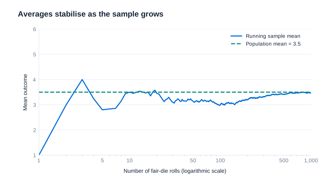
The law of large numbers explains why averages stabilise. For independent, identically distributed observations with a finite expected value, a standard version states:
Convergence in probability means that the probability of a discrepancy larger than any fixed positive tolerance tends to zero as the sample grows. For a fair six-sided die, the expected result is . A running average can fluctuate widely at first and then settle near 3.5. It need not approach 3.5 monotonically, and no universal threshold such as 100 observations guarantees adequate precision.
Sample-size requirements depend on outcome variability, the treatment effect of interest, the assignment scheme and the desired precision. Clustering can reduce the information provided by a nominally large sample because observations within a group may be correlated. Noncompliance, attrition and spillovers can also change the interpretation of an experiment. An effect of assignment to insurance, for example, need not equal the effect of actually receiving insurance if some people do not follow their assignment.
Reading a balance table
A balance table compares characteristics measured before treatment. It helps assess whether assignment groups look comparable and whether implementation or sample attrition has created concerning differences. The RAND Health Insurance Experiment provides an example comparing more generous plans with a catastrophic-coverage plan. The first numerical column below reports the catastrophic group's baseline mean. The other columns report differences from that mean, rather than the alternative groups' means themselves.
| Characteristic | Catastrophic mean | Deductible difference | Coinsurance difference | Free-care difference | Pooled alternative plans difference |
|---|---|---|---|---|---|
| Female share | 0.560 | −0.023 (0.016) | −0.025 (0.015) | −0.038 (0.015) | −0.030 (0.013) |
| Nonwhite share | 0.172 | −0.019 (0.027) | −0.027 (0.025) | −0.028 (0.025) | −0.025 (0.022) |
| Age, years | 32.4 [12.9] | 0.56 (0.68) | 0.97 (0.65) | 0.43 (0.61) | 0.64 (0.54) |
| Education, years | 12.1 [2.9] | −0.16 (0.19) | −0.06 (0.19) | −0.26 (0.18) | −0.17 (0.16) |
| Family income, US dollars | 31,603 [18,148] | −2,104 (1,384) | 970 (1,389) | −976 (1,345) | −654 (1,181) |
| Hospitalised in the previous year, share | 0.115 | 0.004 (0.016) | −0.002 (0.015) | 0.001 (0.015) | 0.001 (0.013) |
| General health index | 70.9 [14.9] | −1.44 (0.95) | 0.21 (0.92) | −1.31 (0.87) | −0.93 (0.77) |
| Cholesterol, mg/dl | 207 [40] | −1.42 (2.99) | −1.93 (2.76) | −5.25 (2.70) | −3.19 (2.29) |
| Systolic blood pressure, mm Hg | 122 [17] | 2.32 (1.15) | 0.91 (1.08) | 1.12 (1.01) | 1.39 (0.90) |
| Mental health index | 73.8 [14.3] | −0.12 (0.82) | 1.19 (0.81) | 0.89 (0.77) | 0.71 (0.68) |
Standard deviations, where reported for the catastrophic group, appear in brackets; standard errors of differences appear in parentheses. Enrolment was 759 in catastrophic coverage, 881 in the deductible plan, 1,022 in coinsurance and 1,295 in free care. The last column pools the 3,198 participants in the three alternative plans. Catastrophic coverage is itself insurance, so this is a comparison of insurance generosity, not a comparison with complete absence of coverage.
For example, the free-care group's female share is approximately . Its baseline general health index is approximately . The table does not show the effect of free care on health: these are baseline characteristics, measured before treatment could produce the subsequent outcomes of interest.
Some baseline differences can be statistically significant by chance, especially when many characteristics are examined. The free-care difference in the female share is about 2.53 standard errors from zero. That observation should be interpreted with the assignment procedure and the full pattern of balance, rather than treated as automatic proof that randomisation failed. Conversely, insignificant differences do not prove that unobserved characteristics are balanced or that there is no important imbalance in a small sample.
The population model and the least-squares solution
When random assignment is unavailable, a regression can describe how an outcome varies with an explanatory variable. The simple linear model is:
Here is the outcome, the explanatory variable, the intercept and the slope. The disturbance collects the outcome's remaining determinants and deviations from the specified relationship. The coefficients are population quantities; their estimates vary across samples. The disturbance is an unobserved random variable, not a fixed population parameter.
Ordinary least squares, or OLS, chooses the intercept and slope that minimise the sum of squared vertical deviations between observed outcomes and the fitted line:
Squaring prevents positive and negative deviations from cancelling and puts greater weight on large discrepancies. Differentiating with respect to the two coefficients gives the normal equations and . Solving them, when varies in the sample, yields:
The denominator is a sum of squared deviations. Without the square, the deviations around the sample mean sum to zero. The slope can equivalently be written as the ratio of sample covariance to sample variance, provided both use the same normalisation. Under the appropriate population orthogonality condition, the corresponding population slope is .
Fitted values, residuals and regression geometry
The fitted value is . The residual is the observed outcome minus this prediction, . It is a vertical distance because the criterion predicts conditional on ; OLS does not minimise perpendicular distances to the line.
In one numerical illustration, the fitted line is and the sum of squared residuals is 384. At , the line predicts 23.07. An observation above that value has a positive residual and one below it a negative residual. The value 384 describes total squared discrepancies in the sample and depends on the outcome's scale and the number of observations; it is not by itself a measure of causal credibility.
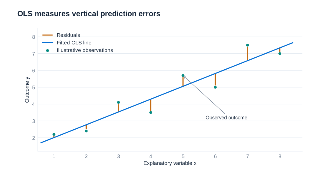
With an intercept, the normal equations imply exact sample identities:
The line therefore passes through , and residuals are orthogonal to the included regressor and fitted values in the sample. These are algebraic properties of the OLS calculation. They do not establish that the population disturbance is unrelated to . An omitted determinant correlated with can bias the coefficient even though the fitted residuals satisfy every one of these identities.
Keeping and distinct prevents a common error. The former belongs to the population model and is not directly observed; the latter is calculated after estimating the model. Inspecting residuals can reveal patterns, unusual observations or inappropriate functional forms, but zero sample covariance between an included regressor and its OLS residuals is guaranteed by construction.
Test scores and the meaning of a slope
A dataset of 420 California school districts relates average test scores to the student-to-teacher ratio. The fitted relationship, using the reported coefficient estimates rounded to two decimal places, is:
The slope associates one additional student per teacher with a 2.28-point lower predicted test score. A reduction in the ratio by two students per teacher corresponds to a 4.56-point increase in the fitted outcome. At a ratio of 20, the prediction is ; at a ratio of 18 it is 657.86. These are predictions from the estimated line, not the observed outcome of every district with those ratios.
Relative to a mean test score of approximately 654, a 2.28-point change is about . This calculation gives scale to the coefficient. It does not make 0.35% the regression coefficient, and it is not a 0.35-percentage-point change. In a linear-linear model, the direct coefficient always measures outcome units per explanatory-variable unit.
The intercept is the predicted outcome when the student-to-teacher ratio is zero, which lies outside the relevant data range. It helps position the fitted line but has little substantive value as a literal prediction. Extrapolating far beyond the observed range is risky because a linear pattern within that range need not continue elsewhere.
Most importantly, the negative slope alone does not show that hiring teachers causes the predicted improvement. District income, language composition and other resources may be associated with both class size and test scores. Regression adjustment can compare districts with similar measured characteristics, but controlling for observables does not automatically eliminate unobserved differences. A causal interpretation requires an argument about the determinants left in the disturbance.
Unbiasedness, consistency and the bias–variance trade-off
An estimator is a rule applied to a sample; an estimate is its realised numerical result. Repeating the sampling process produces a sampling distribution. Unbiasedness means that the average of this distribution equals the population parameter: . It does not mean that every estimate equals the parameter. An unbiased estimator can be imprecise and produce individual estimates far from the truth.
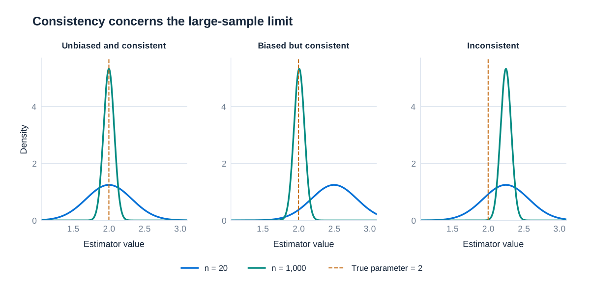
Consistency concerns a sequence of estimators as sample size increases. Formally, . The probability of a fixed-size estimation error then tends to zero. Unlike unbiasedness, consistency is an asymptotic property. More observations do not make an inherently inconsistent procedure consistent; they can instead concentrate its estimates around the wrong value.
Three examples distinguish these concepts. First, suppose satisfies the conditions for unbiased and consistent OLS. The slope distribution is centred on 2 and becomes more concentrated as the sample grows. Second, define a modified estimator . It has finite-sample bias but is consistent when OLS is consistent: the added term is 0.5 at , 0.01 at , and tends to zero.
Third, suppose the disturbance in the same structural equation is , with . Substitution gives . A regression of on converges to 2.25, not the structural coefficient 2. Increasing sample size makes the descriptive slope more precise while leaving the 0.25 discrepancy in the structural interpretation.
Precision and bias are separate dimensions of performance. For a scalar estimator, mean squared error decomposes as:
An estimator with a small bias may have lower mean squared error than a very dispersed unbiased estimator. This trade-off matters when evaluating estimators, but it does not justify ignoring systematic causal bias merely because standard errors are small.
The assumptions behind OLS properties
For the familiar finite-sample unbiasedness result, a central condition is zero conditional mean, , together with a correctly specified linear conditional mean, suitable sampling conditions and variation in . Zero unconditional mean, , is weaker: positive and negative errors can average to zero while still varying systematically with the regressor. Zero covariance between and can support consistency of a linear projection under appropriate regularity conditions, but it should not be presented as equivalent to zero conditional mean.
In multiple regression, the regressors must not be perfectly collinear. In the simple model this means that cannot be constant. Without variation in , the data cannot distinguish the intercept from the slope. Random sampling and finite-moment conditions support laws of large numbers and sampling approximations. Very influential observations require investigation; the formal requirement is not that no unusual observation may exist.
The Gauss–Markov result adds homoskedasticity and absence of correlation between disturbances across observations, conditional on the regressors. Under the relevant assumptions, OLS is the best linear unbiased estimator, or BLUE. “Best” means smallest variance within the class of linear unbiased estimators. “Linear” refers to the estimator being a linear function of observed outcomes, conditional on the regressors. It does not mean that only straight-line relationships can be modelled, nor does it mean that OLS dominates every possible nonlinear or biased estimator.
Normal disturbances are not required for Gauss–Markov. Heteroskedasticity can leave OLS unbiased and consistent under exogeneity while invalidating the usual homoskedastic variance formula and the BLUE claim. Finally, even correct estimation of a conditional association does not automatically establish a causal mechanism: the economic interpretation depends on the research design and the meaning of the disturbance.
What determines precision?
Under homoskedasticity and uncorrelated disturbances, the conditional variance of the simple-regression slope is:
The exact expression conditions on the realised regressor values; the approximation replaces their sum of squared deviations with its large-sample counterpart. Greater disturbance variance makes the line harder to estimate. Greater variation in provides more information about its slope. More observations generally improve precision when they add independent information. The standard error, being the square root of variance, typically decreases at a rate proportional to , so quadrupling sample size approximately halves it under otherwise comparable conditions.
In practice the unknown disturbance variance must be estimated. With an intercept and one slope, a conventional homoskedastic estimator is , giving . The subtraction of two reflects the two estimated coefficients. Heteroskedasticity or dependence requires a variance estimator appropriate to that setting.
Reading a regression result therefore involves three distinct questions. What comparison and units does the coefficient represent? Which assumptions justify interpreting it as the target relationship? How much sampling uncertainty remains? Answering only the first or third can produce an apparently precise conclusion that the design does not support.