
7. Panel Data and Fixed Effects
A panel follows the same units over time. Its distinctive contribution is the ability to compare a person, firm, city or other unit with its own earlier observations. This changes the source of information used by a regression: persistent differences between units can be separated from changes within them. The distinction is valuable whenever an explanatory variable is correlated with stable characteristics that are difficult to measure. It does not, by itself, make an observational relationship causal.
What a panel records
Let identify units and identify periods. An observation is the outcome for unit in period ; is a time-varying explanatory variable. A city panel might record population, capital-city status and the presence of centres of higher learning at successive dates. Longitude is a time-invariant characteristic, written , because its value does not change within the same city. Capital-city status can change, so it belongs among the variables indexed by both and .
A balanced panel observes every unit in every period and contains observations. An unbalanced panel has different numbers of observations across units. This can reflect entry, exit, missing measurements or the historical availability of records. Unbalanced data are not automatically invalid: fixed-effects methods can use the available observations. However, selective disappearance matters. If a firm stops reporting precisely when an unobserved adverse shock occurs, analysing only its observed periods may introduce selection bias. The unit identifier must also remain consistent over time; a changed administrative boundary can create an apparent change that is partly a change in what is being measured.
Repeated cross-sections are different. Observing a new sample of workers every year permits comparisons of groups over time, but does not permit a within-worker transformation unless the same workers can be linked. A panel's repeated observations provide additional information, while also creating dependence: ten measurements of one person are not equivalent to ten independently sampled people.
Why pooled OLS can be misleading
Consider the additive model
The component collects all stable unit characteristics that affect the outcome, including unobserved ones. The idiosyncratic disturbance contains influences that vary over time. A pooled OLS regression that omits combines the two components into one error. Even if the time-varying disturbance is exogenous, a correlation between and creates omitted-variable bias. For instance, a city with a naturally favourable harbour may have both greater commercial activity and a larger population in every period. Comparing high-activity cities with low-activity cities mixes the association of activity with population and the persistent advantage of the harbour.
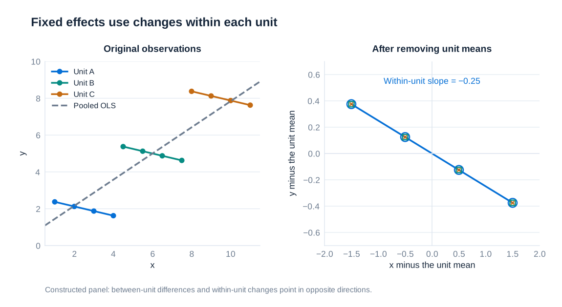
The key distinction is between between-unit variation, represented by differences in unit means, and within-unit variation, represented by deviations from each unit's own mean. A positive pooled relationship can coexist with a flat or negative within-unit relationship. Neither estimate should be interpreted without stating the comparison it uses. Fixed effects deliberately discard persistent level differences as a source of identification for .
The within transformation
For a balanced panel, take each unit's time average. Define , and define and in the same way. The mean of is simply . Subtracting the averaged equation from the original equation gives
Both the common intercept and the unit-specific intercept disappear. OLS on these demeaned variables therefore estimates the slope without requiring to be uncorrelated with . For one explanatory variable, the within estimator is
The denominator shows a fundamental requirement: the explanatory variable must change within at least some units. A variable that is constant within every unit has a demeaned value of zero and cannot receive a separately identified coefficient. This is why a city fixed-effects regression cannot estimate a separate main effect of longitude. Its contribution is absorbed by the city intercept. A small amount of within-unit variation can also lead to imprecise estimates, even when the full dataset contains many observations.
For an unbalanced panel, the average for each unit is calculated over that unit's observed periods, using its own observation count . The algebra remains valid for a time-invariant additive effect. Appropriate assumptions about the observation process are still required for inference about the intended population.
Fixed effects as unit indicators
The same slope can be estimated by giving each unit its own intercept. With a common intercept, include unit indicators; the omitted unit supplies the reference intercept. Alternatively, include all indicators and omit the common intercept. Including both a common intercept and all unit indicators creates perfect multicollinearity because the indicators sum to one for every observation.
The least-squares dummy-variable regression and the within regression produce the same estimated slope when applied to the same observations and regressors. Software must also account correctly for the estimated fixed effects when constructing degrees-of-freedom adjustments. Choosing a different reference unit changes the interpretation of the intercept and indicator coefficients, but does not change fitted values or the slope of the time-varying regressor. Modern estimation routines absorb large collections of fixed effects rather than explicitly constructing thousands of indicator columns.
First differences
Another way to remove is to subtract the previous observation of the same unit:
The fixed effect cancels because . A first-difference regression asks whether a change in the explanatory variable accompanies a change in the outcome. One initial observation per unit is lost when constructing differences. If dates are missing, adjacent recorded rows must not automatically be treated as adjacent periods: a change over two years is not the same object as a one-year change.
With exactly two periods and the same sample, first differences and the within estimator yield the same slope. With more than two periods, both eliminate a fixed additive effect, but their estimates need not coincide. Their relative efficiency depends on the serial structure of the idiosyncratic disturbance. Differencing can also magnify the importance of measurement error when the true variable changes little over time. The choice should therefore reflect the economic model, data quality and error process.
Unit effects and period effects
A two-way fixed-effects model includes both unit and period intercepts:
Unit effects absorb stable differences across units: location, persistent infrastructure advantages or enduring characteristics of an individual. Period effects absorb shocks common to all units at a given date, such as a nationwide recession or a general technological change. For city populations, a common epidemic wave could be represented by a period effect only to the extent that its additive effect is shared across cities. A shock that hits ports more strongly than inland cities is not fully removed by one common time intercept.
In a balanced panel, subtracting unit means and time means and adding the overall mean removes both sets of intercepts. With unbalanced observations, this simple one-step double-demeaning formula is generally insufficient; an estimator that properly absorbs both effects is needed. Variables that move identically for every unit at each date are collinear with time effects. Identification consequently requires variation that remains after both sets of effects have been removed.
Exogeneity, serial dependence and inference
A standard sufficient condition for the static fixed-effects estimator is strict exogeneity of the idiosyncratic disturbance:
This condition permits correlation between the regressors and the stable effect , but rules out correlation between a disturbance in one period and regressors in any period. It is stronger than contemporaneous exogeneity. If an unexpected fall in city population causes the government to introduce a policy next period, the current shock is related to a future regressor. Removing the city mean does not remove this feedback. Time-varying omitted factors, simultaneous determination and endogenous measurement remain possible sources of bias. Lagged dependent variables require particular care in short panels because the within transformation generally makes them correlated with the transformed disturbance.
Repeated observations also create an inference problem. After fixed effects have been removed, idiosyncratic shocks can still be persistent within units. Cluster-robust standard errors allow heteroskedasticity and serial correlation within a specified cluster while relying on adequate independence across clusters. If policy varies by state, clustering only by individual can substantially understate uncertainty: many individuals share the same policy shock. The clustering level should follow the assignment mechanism and plausible common disturbances, and the number of independent clusters matters more than the raw number of rows. Clustered standard errors address uncertainty; they do not repair an endogenous regressor.
Random effects and the source of identifying variation
A random-effects model also separates from , but uses both within-unit and between-unit information. In its conventional form it requires the unit effect to be uncorrelated with the regressors at all dates, conditional on included controls. This assumption is demanding when, for example, unobserved management quality influences both a firm's investment and its output. If the assumption is credible, random effects can improve efficiency and estimate coefficients on time-invariant regressors that fixed effects absorb.
Random effects are therefore a substantive modelling choice, not an obsolete method. Correlated random-effects approaches can relax the conventional assumption by explicitly including functions of a unit's regressor history, such as time averages. A comparison of fixed- and random-effects estimates can be informative, but an automated test cannot establish the economic credibility of all identifying assumptions. Above all, a table containing coefficients for time-invariant geography cannot be described as a standard city fixed-effects regression that also estimates those geography main effects.
Long-run city development: reading an empirical table
Bosker, Buringh and van Zanden's study of urban development between 800 and 1800 assembles information on 793 cities across Europe, the Middle East and North Africa. The setting distinguishes stable geography from changing institutions. Sea access and transport networks can influence commerce, while political and religious status can change a city's administrative or economic role. Historical coverage and variable availability mean that individual regression samples need not contain every city at every date.
The following baseline table is a random-effects specification with additional ecozone, country and century fixed effects. It is not the city fixed-effects specification developed above. The dependent variable is the natural logarithm of city population. Each reported cell gives a coefficient followed by its city-clustered p-value in brackets. A displayed p-value of 0.00 is a rounded small value, not a probability known to be exactly zero. “Not included” identifies a variable not estimated in that specification rather than a missing result.
| Characteristic | All cities | Muslim cities | Christian cities | Middle East / North Africa | Europe | Muslim cities: Middle East / North Africa | Christian cities: Europe |
|---|---|---|---|---|---|---|---|
| Sea access | 0.25*** [0.00] | 0.24 [0.11] | 0.25*** [0.00] | 0.42*** [0.01] | 0.26*** [0.00] | 0.38** [0.04] | 0.25*** [0.00] |
| River access | 0.09** [0.04] | 0.12 [0.23] | 0.05 [0.31] | 0.21* [0.07] | 0.06 [0.25] | 0.11 [0.42] | 0.05 [0.3] |
| Roman road | 0.03 [0.59] | −0.09 [0.55] | 0.06 [0.22] | 0.08 [0.71] | 0.03 [0.61] | 0.05 [0.84] | 0.05 [0.28] |
| Roman-road hub | 0.09* [0.10] | 0.08 [0.54] | 0.10** [0.04] | 0.12 [0.55] | 0.08 [0.13] | 0.12 [0.57] | 0.10** [0.05] |
| Caravan route | 0.08 [0.46] | 0.31* [0.05] | −0.34*** [0.00] | 0.06 [0.66] | Not included | 0.25 [0.15] | Not included |
| Caravan hub | 0.5*** [0.00] | 0.78*** [0.00] | 0.09 [0.61] | 0.55*** [0.00] | Not included | 0.70*** [0.00] | Not included |
| Bishopric | 0.18*** [0.00] | 0.22** [0.04] | 0.19*** [0.00] | 0.37*** [0.00] | 0.17*** [0.00] | 0.27* [0.06] | 0.19*** [0.00] |
| Archbishopric | 0.34*** [0.00] | 0.12 [0.45] | 0.41*** [0.00] | 0.35 [0.16] | 0.39*** [0.00] | 0.22 [0.36] | 0.41*** [0.00] |
| Christian holy city | 0.26 [0.26] | Not included | 0.47 [0.12] | 0.29 [0.57] | 0.22 [0.54] | Not included | 0.34 [0.34] |
| Muslim holy city | 0.19 [0.24] | −0.08 [0.79] | Not included | 0.02 [0.93] | Not included | −0.18 [0.62] | Not included |
| Capital city | 0.87*** [0.00] | 0.67*** [0.00] | 0.93*** [0.00] | 0.73*** [0.00] | 0.91*** [0.00] | 0.72*** [0.00] | 0.95*** [0.00] |
| Centre of higher learning | 0.32*** [0.00] | 0.09 [0.83] | 0.30*** [0.00] | 0.11 [0.75] | 0.29*** [0.00] | 0.16 [0.74] | 0.30*** [0.00] |
| Madrasa | 0.25** [0.01] | 0.12 [0.25] | Not included | 0.19 [0.11] | 0.12 [0.48] | 0.16 [0.19] | Not included |
| Plundered | 0.03 [0.56] | 0.02 [0.57] | −0.09 [0.14] | 0.07 [0.103] | −0.16*** [0.01] | 0.03 [0.41] | −0.14** [0.03] |
| Log Muslim urban potential | 0.08 [0.31] | 0.30** [0.04] | 0.03 [0.72] | 0.24 [0.12] | 0.19** [0.04] | 0.29* [0.10] | 0.07 [0.47] |
| Log Christian urban potential | 0.23*** [0.00] | 0.29 [0.12] | 0.25*** [0.00] | −0.02 [0.9] | 0.21*** [0.00] | 0.18 [0.43] | 0.25*** [0.00] |
| R² | 0.46 | 0.52 | 0.43 | 0.60 | 0.40 | 0.56 | 0.41 |
| Observations | 2,596 | 656 | 1,940 | 570 | 2,026 | 499 | 1,869 |
Dependent variable: natural log of city population. Brackets contain p-values based on standard errors clustered by city. Significance markers are reproduced at their reported precision: * 10%, ** 5%, *** 1%. All specifications allow city random effects and include ecozone, country and century fixed effects. Additional controls cover religion where applicable, relevant logged distances to Mecca, Byzantium and Rome, log elevation, log surrounding ruggedness and cultivation potential. The centre-of-higher-learning indicator and madrasa indicator distinguish the two institutional categories used in the study.
Transport patterns differ across subsamples: sea access has a positive association in most specifications, while caravan networks have especially strong associations in Muslim-city samples. The measures of urban potential distinguish access to Muslim and Christian city networks; their log coefficients are elasticities conditional on the model. Capital status is positively associated with population throughout the table. Religious administrative status and centres of learning also show positive associations in several samples. These findings describe conditional relationships, not automatic proof of causal institutional effects. A growing city may acquire a political or educational institution because it is already expanding.
The interpretation depends on functional form. A capital coefficient of 0.87 corresponds to a fitted population ratio of , or about 139% more in the exponentiated log specification, rather than 87% exactly. For a log urban-potential variable, a coefficient of 0.23 instead means that a 1% change in urban potential is associated approximately with a 0.23% change in population. Such exponentiation describes fitted ratios on the log scale; translating them into arithmetic conditional mean populations can additionally require a retransformation adjustment when the disturbance distribution changes across observations.
Interpreting time indicators correctly
With the year 800 omitted, a century coefficient compares a period with that reference period, conditional on the other regressors. The table below is a coefficient-interpretation example. Its stated sample has 8,723 observations, so it must not be conflated with the 2,596-observation baseline above. Only reported centuries are listed; no estimates are supplied for omitted entries in the example.
| Century | Log coefficient | t-statistic |
|---|---|---|
| 800 | Reference period | Not estimated |
| 900 | 0.299 | 1.89 |
| 1000 | 0.845*** | 5.35 |
| 1100 | 0.963*** | 6.10 |
| 1200 | 1.553*** | 9.83 |
| 1300 | 3.006*** | 19.03 |
| 1400 | 2.224*** | 14.08 |
| 1700 | 4.955*** | 31.37 |
| 1800 | 8.036*** | 50.87 |
Year 800 is the omitted category. The example does not report coefficients for 1500 or 1600. Three stars denote significance at the 1% level.
In a log-outcome model, is a small-coefficient approximation to a percentage difference. The exact exponentiated comparison is . Thus 0.299 implies approximately 34.9%, while 0.845 implies approximately 132.8%. At 8.036, the approximation is entirely inappropriate: the corresponding fitted ratio is about 3,090.2, not a population difference of 803.6%. The exceptionally large value illustrates why a result's scale and provenance must be checked before giving it a substantive historical interpretation.
Changing effects of geography and institutions
Although the main effect of a time-invariant characteristic is absorbed by unit effects, its interaction with time can be identified. Suppose records coastal access. In a city and time fixed-effects model, include interacted with each period indicator except the reference year. A coefficient then measures how the coastal–inland difference changed relative to that reference year, rather than the overall difference in that year.
| Century | Interaction coefficient |
|---|---|
| 800 | Reference period |
| 900 | 0.14 |
| 1000 | 0.09 |
| 1100 | 0.02 |
| 1200 | −0.03 |
| 1300 | 0.12 |
| 1400 | 0.02 |
| 1500 | 0.11 |
| 1600 | 0.27 |
| 1700 | 0.38** |
| 1800 | 0.45** |
City and period fixed effects are included. Two stars denote significance at the 5% level. Standard errors and t-statistics are not provided in this example.
The coefficient 0.45 for 1800 is an additional 0.45 log points in the coastal–inland gap relative to 800. Exponentiating gives a ratio-of-ratios of , or about a 56.8% increase in that relative ratio. It is not automatically a 45-percentage-point difference in ordinary population growth rates. Such a percentage-point statement would require additional information about the baseline and growth rates being compared.
A time-varying characteristic can be interacted with all period indicators when the separate overall main effect is omitted and the design matrix has sufficient rank. For capital status, this parameterization estimates a period-specific coefficient directly. If instead one includes an overall capital coefficient plus interactions for all but the reference period, the interactions become deviations from that reference coefficient. These are alternative parameterizations of the same fitted relationships, not competing economic theories.
| Century | Capital-status coefficient |
|---|---|
| 800 | 0.19 |
| 900 | 0.50 |
| 1000 | 0.41 |
| 1100 | 0.40*** |
| 1200 | 0.48*** |
| 1300 | 0.47*** |
| 1400 | 0.45*** |
| 1500 | 0.61*** |
| 1600 | 0.63** |
| 1700 | 0.82** |
| 1800 | 0.64* |
City and period fixed effects are included. Significance: * 10%, ** 5%, *** 1%. Standard errors and t-statistics are not provided in this example.
For example, a period-specific capital coefficient of 0.64 corresponds to an exponentiated conditional difference of about 89.6%. Whether this deserves a causal interpretation still depends on why capital status changed and whether relevant time-varying confounders were controlled. Interactions expand the model's flexibility, but they do not create exogenous variation.
Evaluating a panel result
A useful assessment begins by identifying the unit, period and actual estimation sample. It then asks which variables change within units, which effects are absorbed, and what remaining variation identifies the coefficient. The economic story must explain why that variation is unrelated to the idiosyncratic disturbance. Finally, the uncertainty calculation must respect the dependence induced by repeated observations and shared shocks. Panel data help remove a specific class of omitted variables—stable additive unit characteristics—but a credible causal design must also address the confounders that remain.