
6. Dummy Variables and Binary Outcomes
Indicators, categories and the comparison they encode
A binary or dummy variable takes the value 1 when a defined condition holds and 0 otherwise. Employment status, an apartment’s ocean view and the presence of high blood pressure are examples. Binary variables are a special case of categorical variables, which classify observations into a limited set of groups. The coding must be stated explicitly: reversing 0 and 1 reverses the interpretation of the associated comparison.
A numeric category code is not necessarily a quantitative measurement. Coding blood types A, B, AB and O as 1, 2, 3 and 4 does not make type O “four times” type A, nor establish equally spaced biological differences. Treating these codes as one continuous regressor would impose an arbitrary ordering and constant steps. Separate indicators allow each group to have its own conditional mean relative to a chosen reference category.
There are two distinct uses of binary variables in regression. An indicator on the right-hand side represents a group comparison while leaving the nature of the outcome unchanged. An indicator on the left-hand side makes the conditional mean a probability, introducing restrictions that an ordinary straight line may fail to respect. The estimation principles remain connected, but the interpretation and appropriate diagnostics differ.
A dummy variable as an explanatory variable
Suppose monthly apartment rent, in currency units, is modelled using the number of rooms and an ocean-view indicator:
For a fixed room count, the fitted rent is without an ocean view and with a view. Thus is the conditional difference in monthly rent, measured in the same currency units as rent. The model assumes that this difference does not vary with the number of rooms. Adding would relax that restriction, allowing the view premium to vary with apartment size.
“Holding rooms constant” does not mean all other apartment characteristics are identical. If ocean-view properties also have better locations or higher construction quality and those variables are omitted, the coefficient may reflect those differences. The group indicator does not supply random assignment. Its coefficient is a conditional association unless the identifying assumptions justify more.
If the dependent variable is log rent, the coefficient changes meaning: the exact fitted proportional difference between view and no-view apartments is %, subject to the logged-outcome qualifications in Chapter 5. If an indicator interacts with another regressor, its standalone coefficient applies when that other regressor is zero, and the full group contrast must include the interaction.
Multiple categories and the dummy-variable trap
Consider a school-district example that groups computer availability into low, middle and high categories using the 25th and 75th percentiles. To define a complete classification, assign values below the 25th percentile to low, values from the 25th through the 75th percentile to middle, and values above the 75th percentile to high. Ties require a consistent boundary rule; the groups need not contain exactly 25%, 50% and 25% of observations.
Let and indicate middle and high availability. With low availability as the reference, estimate:
The intercept is the low group’s mean, and the two slopes are differences relative to it. Including all three group indicators together with an intercept produces perfect multicollinearity because their sum is exactly 1. This is the dummy-variable trap. Omitting one category with an intercept solves it; alternatively, omitting the intercept and retaining all categories estimates separate group means. Neither option discards observations from the reference group.
| Term | Coefficient | Standard error | t statistic | p value | 95% confidence interval |
|---|---|---|---|---|---|
| Middle versus low | 0.8566319 | 2.275697 | 0.38 | 0.707 | [−3.616636, 5.3299] |
| High versus low | −0.9260766 | 2.627719 | −0.35 | 0.725 | [−6.091303, 4.23915] |
| Intercept: low category | 653.9618 | 1.85367 | 352.79 | <0.001 | [650.3181, 657.6055] |
The fitted means are approximately 653.96 points for low availability, 654.82 for middle availability and 653.04 for high availability. Both difference intervals include zero. The joint test of the two category coefficients gives , with ; , adjusted , and the root mean squared error is 19.085 score points. These results provide little evidence of differences in this simple grouping. They do not prove that access to computers has no causal effect: the specification is an unadjusted group comparison, and the measure is computer availability rather than a randomly assigned intervention.
Binary outcomes and the linear probability model
For a binary outcome , its conditional expectation equals its probability of being 1: . Running OLS with a binary outcome therefore gives a linear probability model, or LPM. In , a one-unit increase in changes the fitted probability by , or percentage points. The scale is essential: a coefficient of 0.05 means five percentage points, not automatically a 5% relative increase.
For school districts, define when the district’s average test score is above the chosen overall average and 0 otherwise. A regression on average district income produces the following results. Income is kept in the dataset’s recorded units, so the slope applies to one unit on that scale; any currency conversion must be applied before interpreting a different unit change.
| Term | Coefficient | Robust standard error | t statistic | p value | 95% confidence interval |
|---|---|---|---|---|---|
| Average district income | 0.0328825 | 0.0029316 | 11.22 | <0.001 | [0.0271201, 0.038645] |
| Intercept | 0.0034945 | 0.0504409 | 0.07 | 0.945 | [−0.095655, 0.102644] |
There are 420 observations; , root mean squared error 0.44108, and the robust overall test is , with . A one-unit income increase is associated with about 3.288 percentage points higher probability of an above-average score. This comparison is about crossing a binary threshold, not the number of test-score points gained.
Probability bounds, heteroskedasticity and percentage points
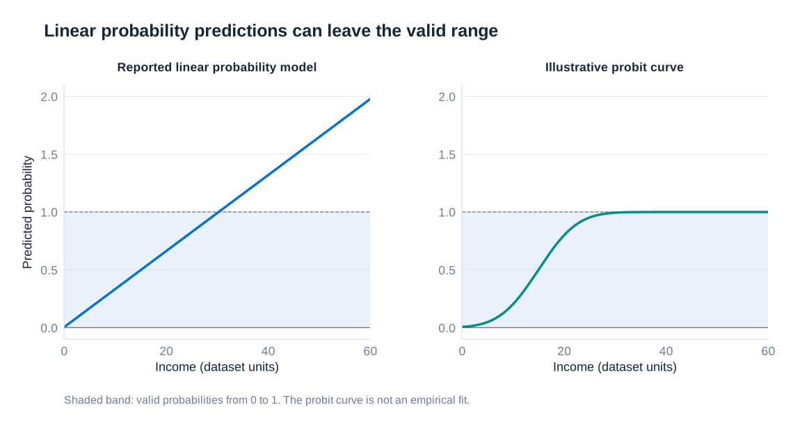
A straight line need not stay between 0 and 1. The fitted school model is , which exceeds 1 when recorded income exceeds approximately 30.31. At , it predicts about 1.319, an impossible probability. Such predictions reveal a limitation of the functional form; merely truncating them to 1 does not change the model that was estimated or provide a principled marginal-effect calculation.
The LPM also imposes a constant probability slope. An income increase has the same fitted effect near a probability of 0.05 as near 0.95, although the room for further decreases or increases is very different. The importance of this restriction depends on the range of covariates and the purpose of the analysis. A linear approximation may be useful over a central range even if it behaves badly in the tails.
With a correctly specified conditional probability , the binary error variance is . It therefore generally varies with the regressors, making heteroskedasticity-robust standard errors appropriate. Robust inference addresses this variance problem; it does not repair impossible probabilities, omitted variables or an incorrect conditional mean. If observations are dependent within groups, the standard-error calculation must address that dependence as well.
Percentage points and percent changes answer different questions. A probability moving from 40% to 50% increases by 10 percentage points and by 25% relative to its starting value, because . In a group of fixed size 100, moving from 40 to 50 members with a characteristic illustrates both statements. Without a baseline probability, an LPM coefficient cannot be converted into a unique relative percentage change.
Probit, logit and maximum likelihood
Probit and logit replace the unrestricted probability line with a smooth cumulative distribution function. With an index , the probit model uses the standard normal cumulative distribution function :
The function is the area under the standard normal density to the left of . It maps every real-valued index into a probability strictly between 0 and 1 for finite values. The logit model uses the logistic function instead:
Both curves flatten near their lower and upper bounds. The raw coefficients describe changes in an index, not percentage-point changes in probability. For a continuous regressor without interactions, the probit marginal effect is , where is the standard normal density; the logit marginal effect is . Their magnitude depends on all covariates through the index. An average marginal effect averages these observation-specific derivatives, while an effect evaluated at average covariates is a different quantity.
For a binary regressor, calculate the discrete difference between predicted probabilities when its value is set to 1 and to 0, holding other covariates fixed. Interactions require still more care: the sign of a coefficient on a product term need not by itself equal the sign of every probability-scale interaction effect. Presenting fitted probabilities or explicitly calculated contrasts is often clearer.
These models are usually estimated by maximum likelihood rather than OLS. For independent observations with probabilities , the binary log-likelihood is:
Maximisation selects the parameter values that give the observed outcomes the greatest likelihood within the specified model. Probit, logit and LPM predictions can be similar over a central range, but this is not guaranteed, especially in the tails. Choose between them by considering the target comparison, predicted probability range, specification and interpretability. A nonlinear probability model supplies sensible bounds, not a causal research design.
Reading a complete regression output
A coefficient table contains several distinct pieces of information. The coefficient gives an estimated conditional relationship in the model’s units. Its standard error measures sampling uncertainty under the chosen variance estimator. A test statistic compares the estimate with a hypothesised value, usually zero; the p value describes compatibility with that null under the testing assumptions. A 95% confidence interval summarises a range generated by a procedure with 95% long-run coverage. Neither the p value nor the interval measures the probability that a particular causal story is true.
The number of observations states the sample actually used. is the fraction of sample outcome variation explained by the fitted regression; adjusted penalises added regressors and may be negative. Root mean squared error expresses residual spread in the dependent variable’s units. The overall F test assesses a joint restriction on slope coefficients. None of these statistics substitutes for substantive effect sizes, a valid research design or a careful description of the sample.
| Conditional relationship | Comparison | Interpretation of the fitted change |
|---|---|---|
| One more unit of | units of | |
| One more unit of | Approximately %; exact fitted log-scale comparison % | |
| 1% more | Approximately outcome units; exactly | |
| 1% more | Approximately %; is the elasticity | |
| Binary , linear probability model | One more unit of | percentage points |
Logged-outcome comparisons refer directly to fitted log values and their implied geometric means; arithmetic-mean comparisons require the retransformation conditions discussed in Chapter 5. Every interpretation also holds the other included regressors fixed and remains associational unless additional assumptions establish causality.
Worked example: annual medical expenditure in levels
Three models use 2,970 observations and the same explanatory variables: age in years, the natural logarithm of personal income, and an obesity indicator equal to 1 for obese individuals and 0 otherwise. The first outcome is total annual medical expenditure measured in 2005 US dollars. Its coefficients therefore combine three interpretation rules: a level–level age effect, a level–log income effect and a discrete group difference.
| Term | Coefficient | Standard error | t statistic | p value | 95% confidence interval |
|---|---|---|---|---|---|
| Age, years | 202.1078 | 43.41592 | 4.66 | <0.001 | [116.9794, 287.2362] |
| ln(personal income) | −260.2222 | 772.2026 | −0.34 | 0.736 | [−1774.329, 1253.885] |
| Obese indicator | 1251.303 | 588.4134 | 2.13 | 0.034 | [97.56308, 2405.043] |
| Intercept | −4462.544 | 7241.433 | −0.62 | 0.538 | [−18661.29, 9736.197] |
Holding income and obesity status fixed, an additional year of age is associated with approximately USD 202.11 higher annual expenditure. A 1% income increase corresponds to approximately USD 2.60 lower expenditure, because the coefficient multiplies the change in log income; the exact fitted change is . The income estimate is very imprecise and its interval includes substantial positive and negative values, so the negative point estimate should not be presented as established evidence that income reduces expenditure.
At the same age and income, the obese group has fitted annual expenditure USD 1,251.30 higher. Its interval ranges from approximately USD 97.56 to USD 2,405.04. The intercept describes a non-obese individual at age zero and log income zero, meaning income equal to one in the recorded currency unit. This combination is generally not substantively representative; a negative intercept does not imply negative expenditure for a typical person.
The regression has , adjusted and root mean squared error 14,058 USD. The joint test gives , with . Statistical evidence of some association can coexist with low explanatory power and large individual prediction errors. The estimates do not isolate causal effects of ageing, income or obesity without further assumptions about omitted health conditions, selection and other determinants of expenditure.
Worked example: medical expenditure in logarithms
The second model uses the natural logarithm of annual expenditure. It therefore concerns proportional expenditure differences and requires positive expenditure observations for the logarithm to be defined. Although the reported sample size remains 2,970, one should never assume that an arbitrary dataset contains no zero expenditure merely because a logged specification is convenient.
| Term | Coefficient | Standard error | t statistic | p value | 95% confidence interval |
|---|---|---|---|---|---|
| Age, years | 0.0419183 | 0.0058171 | 7.21 | <0.001 | [0.0305124, 0.0533243] |
| ln(personal income) | −0.1696737 | 0.1034636 | −1.64 | 0.101 | [−0.3725414, 0.0331939] |
| Obese indicator | 0.420106 | 0.0788386 | 5.33 | <0.001 | [0.2655222, 0.5746899] |
| Intercept | 6.448543 | 0.9702434 | 6.65 | <0.001 | [4.546125, 8.350962] |
The age coefficient corresponds to approximately 4.19% higher expenditure per additional year, or an exact fitted geometric-mean difference of %. The income coefficient is an elasticity: a 1% income increase is associated with approximately 0.170% lower expenditure, holding age and obesity status fixed. The exact finite-change figure is about −0.169%. Its confidence interval includes zero and the p value is 0.101, so the data do not establish a nonzero income association at the conventional 5% level.
The obesity coefficient is large enough that the common small-coefficient approximation is misleading. The exact fitted difference is %, rather than 42%. This compares conditional geometric means. Describing it as a 52.21% difference in arithmetic mean expenditure would additionally require an appropriate retransformation assumption or calculation. The intercept is the fitted log expenditure for the baseline covariate combination, not expenditure in dollars.
The model reports , adjusted , root mean squared error 1.8836 log units and , with . Its cannot be compared directly with Model 1’s to decide which better predicts dollar expenditure, because the dependent variable and residual scale have changed.
Worked example: the probability of high blood pressure
The third outcome equals 1 if an individual has high blood pressure and 0 otherwise. OLS therefore estimates an LPM. The age and obesity coefficients describe probability differences; the income coefficient combines a probability outcome with a logged regressor.
| Term | Coefficient | Standard error | t statistic | p value | 95% confidence interval |
|---|---|---|---|---|---|
| Age, years | 0.0053784 | 0.001421 | 3.79 | <0.001 | [0.0025922, 0.0081646] |
| ln(personal income) | 0.0914678 | 0.0252735 | 3.62 | <0.001 | [0.0419125, 0.1410232] |
| Obese indicator | 0.1987462 | 0.0192582 | 10.32 | <0.001 | [0.1609854, 0.2365071] |
| Intercept | −0.6557299 | 0.2370055 | −2.77 | 0.006 | [−1.120442, −0.191018] |
An additional year of age is associated with percentage points higher probability. A 1% income increase changes the fitted probability by approximately , or 0.0914678 percentage points. Using the exact log change gives about 0.0910135 percentage points. Multiplying by 100 without also accounting for the 0.01 log change would overstate this comparison by a factor of 100.
The obese group has an estimated probability 19.87462 percentage points higher, conditional on age and income. This is not a 19.87% relative increase: the relative figure would require a specified baseline probability. The negative intercept illustrates again why a baseline outside the useful data range is not a plausible standalone probability. Predictions should be examined over the actual covariate values.
The output reports , adjusted , root mean squared error 0.46012 and , with . The displayed standard errors are conventional OLS standard errors, unlike the explicitly robust school-district example. Given the binary outcome, a sound empirical analysis should recompute heteroskedasticity-robust or otherwise appropriate uncertainty before relying on these reported tests. The coefficient interpretations remain as stated, but their statistical precision must be assessed using an adequate variance estimator.