
8. Impulse responses, shocks and simulated business cycles
Introduction
A calibrated solution becomes economically meaningful when its responses can be interpreted. An impulse response function (IRF) starts at steady state, introduces one innovation and computes the subsequent path of output, consumption, labor, capital and investment. Repeating the recursion explains how persistence in technology and the capital stock turns a one-period shock into a multi-period adjustment.
With a positive technology shock, current output and the wage rise. Consumption smoothing prevents households from consuming the entire extra product immediately; much of the increase may be invested, while the return to working also changes labor supply. A separate capital-stock experiment has different timing precisely because the production function uses capital inherited from the previous period.
To evaluate the model quantitatively, simulate a sequence of innovations, construct artificial time series, filter them consistently with the real data and compare relative standard deviations and correlations. A close qualitative match is informative, but discrepancies—especially in relative volatilities—indicate where the basic RBC model is incomplete.
Integrated theoretical explanation
An impulse response function traces the equilibrium effect of a controlled innovation. The analysis starts from the deterministic steady state, introduces a shock at date zero, and computes the subsequent deviations of the variables while setting later innovations to zero. This isolates the model's propagation mechanism from the randomness of other disturbances. The response at each date is calculated using the previously installed capital stock, the current productivity state and the policy functions obtained from the linear rational-expectations solution.
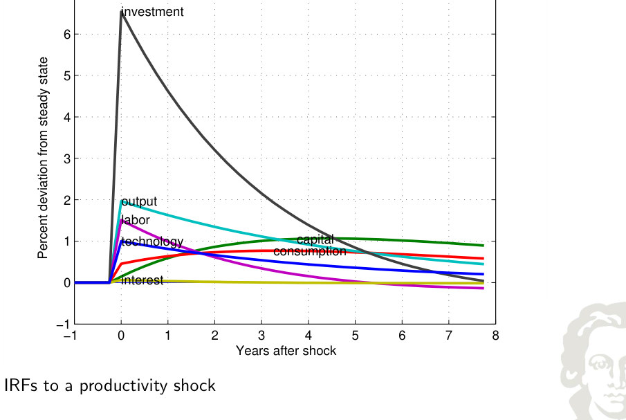
Consider a one-percent innovation to log productivity when initial capital equals its steady-state value. The impact effect comes from multiplying the relevant technology-loading coefficient by the shock. Under the calibrated decision rules, output increases by about 1.97 percent, hours by about 1.52 percent, consumption by about 0.45 percent, and investment by about 6.52 percent; the installed capital chosen for the following period rises by about 0.15 percent. The different magnitudes are not contradictory: consumption is smoothed, while investment absorbs a relatively large fraction of the output adjustment and can consequently be much more volatile.
At the next date the technology deviation equals ρ times its previous value if there are no new innovations. But the economy also inherits the extra capital created by investment in the preceding period. Each policy function therefore has two drivers, one arising from the still-persistent productivity state and the other from endogenously accumulated capital. The capital channel can prolong the response even as the direct productivity disturbance fades. Recursively applying the transition equations gives a complete path for output, consumption, hours, capital and investment, rather than only the one-period effect.
The economic interpretation begins with increased productive capacity. A positive productivity innovation raises output and the marginal product of labor at a given factor allocation. Households respond to higher wages and expected capital returns; in the benchmark, work and investment rise on impact. Because an additional unit of consumption today has diminishing marginal value and households expect some of the disturbance to be temporary, they prefer to distribute part of the gains across future dates. Saving transforms the initial disturbance into additional future capital and therefore links current labor and output decisions to subsequent production possibilities.
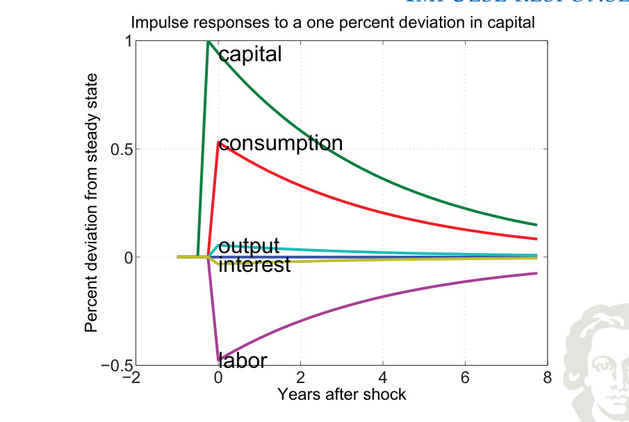
A deviation in installed capital is a different experiment. Here the initial change concerns the economy's predetermined productive asset rather than the technology process. The precise time convention matters: capital inherited at the start of a period is usable during that period, whereas newly chosen investment is not productive until subsequently. A higher capital stock affects marginal products, wages and household wealth differently from a favorable productivity innovation, so the induced responses of hours and investment need not have the same signs or magnitudes. The experiment helps separate propagation through accumulation from propagation through the technology process.
Single-shock responses do not measure whether the economy exhibits realistic variability during an extended sample. Simulation repeatedly draws innovations from the assumed technology process, applies the recursive decision rules, and generates synthetic time series. These series can be HP-filtered or otherwise transformed with the same settings used for observed data. The resulting volatilities, relative volatilities and correlations describe what the model predicts for the distribution of cyclical movements across many periods, conditional on its structure and parameters.
The comparison with observed moments gives a mixed but informative assessment. For the benchmark calibration, investment is much more volatile than output and consumption is smoother; consumption, investment and hours tend to move positively with output. Those features resemble the stylized business-cycle facts. However, the benchmark can underpredict the relative amplitude of important variables and imply correlations that are too strong. A model reproducing the direction of comovement has not thereby explained every recession or established productivity as the only relevant disturbance. It has identified one coherent mechanism whose quantitative strengths and limits can be evaluated.
The distinction between mechanism and policy conclusion is especially important here. The baseline RBC environment has flexible prices and no explicit monetary policy authority or nominal pricing problem, so it cannot on its own supply a full theory of inflation stabilization or nominal interest-rate interventions. Evaluating those questions requires a model with the relevant additional structure. The broader DSGE program extends the discipline of optimal decisions, forward-looking expectations and market consistency rather than replacing it. The RBC analysis supplies a foundation, not a complete account of all policy instruments.
Formal framework and essential relationships
With no further innovations, the technology state decays deterministically at rate ρ. Endogenous capital adds a second channel of persistence beyond the technology process itself.
These impact responses follow from the rounded policy coefficients with initial capital at steady state, k̂₋₁ = 0, and a one-percent productivity innovation, ẑ₀ = 1%. Investment responds much more strongly than consumption in this calibration.
| Variable | Model relative volatility | Data relative volatility | Model corr. with Y | Data corr. with Y |
|---|---|---|---|---|
| Output | 1.0 | 1.0 | 1.00 | 1.00 |
| Technology | 0.8 | 0.5 | 1.00 | not reported |
| Consumption | 0.3 | 0.5 | 0.87 | 0.77 |
| Investment | 3.3 | 4.8 | 0.99 | 0.91 |
| Hours | 0.5 | 0.7 | 0.98 | 0.85 |
For the reported moments, the benchmark reproduces stronger investment than consumption fluctuations and positive comovement, while understating several relative volatilities. The comparison is illustrative: sample periods, definitions and filters must match before interpreting differences as model failures.
Explanations, derivations and empirical applications
RBC Model Analysis
An impulse-response experiment combines technology persistence with capital accumulation. Repeated simulation then generates model-based volatilities and correlations, making possible a systematic comparison with observed business-cycle data.
The analysis has two complementary goals. First, trace how an individual technology innovation propagates to output, consumption, investment and hours with all subsequent innovations set to zero. Second, simulate many shocks and compare the relative volatilities and correlations of the resulting artificial series with their empirical counterparts. Impulse responses explain the mechanism; simulated moments test its quantitative implications.
Impulse Response Functions
A date-zero response can be calculated from the shock loading alone when inherited capital starts at steady state. Later responses require both the persisting productivity state and the additional capital installed through previous investment.
Starting at steady state with an inherited capital deviation of zero, introduce a one-percent log-productivity innovation. The first-period response of each control is its productivity-loading coefficient multiplied by the shock. In the calibrated example, output and hours react strongly, consumption moves less and investment reacts disproportionately. Subsequent dates require updating both productivity through its autoregression and capital through the endogenous transition equation.
Economic propagation and quantitative assessment
A positive productivity innovation raises output and the marginal product of labor for given factor inputs. Consumption smoothing directs part of the additional output into investment, which raises future productive capital. Under the benchmark calibration the wage substitution effect also increases hours, amplifying output. These responses are equilibrium implications of the calibration, not universal signs under every preference specification.
Impulse Response
Fit to text
Scroll horizontally to inspect the labels and values.
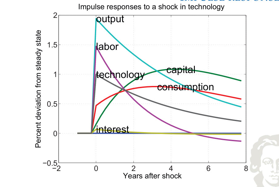
The path traces deviations after the initial disturbance, holding later innovations at zero. The shape results from current factor decisions, persistent productivity and the capital accumulated in previous periods; the response should be interpreted as an equilibrium deviation rather than a forecast of calendar-date data.
Fit to text
Scroll horizontally to inspect the labels and values.
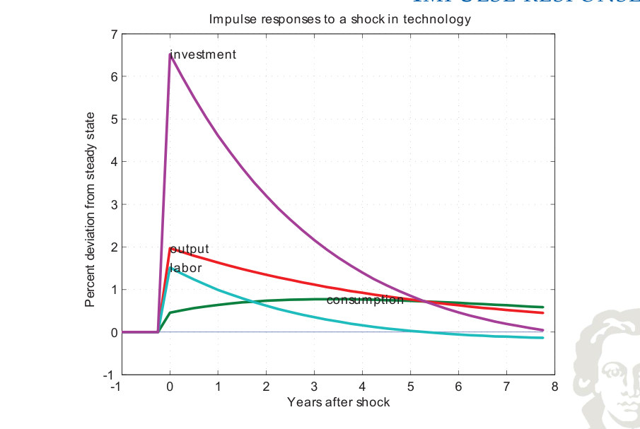
Impulse responses to a shock in technology
Fit to text
Scroll horizontally to inspect the labels and values.
Economic propagation and quantitative assessment
A separate experiment introduces a one-percent deviation in inherited capital k₋₁, with productivity initially at steady state. Its response differs from the experiment that changes productivity at date zero.
Impulse Response
Fit to text
Scroll horizontally to inspect the labels and values.
Fit to text
Scroll horizontally to inspect the labels and values.
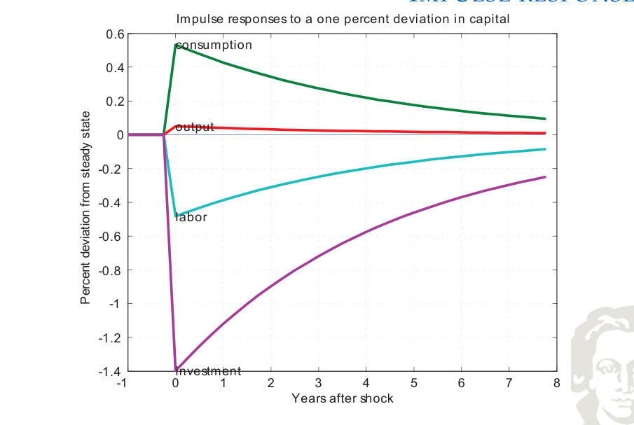
A Capital Stock Shock
A change in installed capital is propagated through different prices and incentives than a productivity innovation. Extra capital affects the marginal product of labor, the return on capital and the household’s future resources. The timing of capital availability is decisive: capital chosen as current investment is installed for subsequent production. The resulting transition highlights the importance of predetermined state variables.
Economic propagation and quantitative assessment
The model–data comparison evaluates relative standard deviations and cross-correlations, not merely the visual similarity of sample trajectories. It is important to apply compatible filtering rules to real and simulated series.
The quantitative comparison considers both dispersion and comovement. Relative standard deviations show that investment should fluctuate much more than output while consumption moves more smoothly; correlations summarize whether consumption, investment and hours are procyclical. A plausible sign pattern does not guarantee an exact empirical fit, and remaining deviations point toward mechanisms omitted from the benchmark.
Simulated Data
Fit to text
Scroll horizontally to inspect the labels and values.
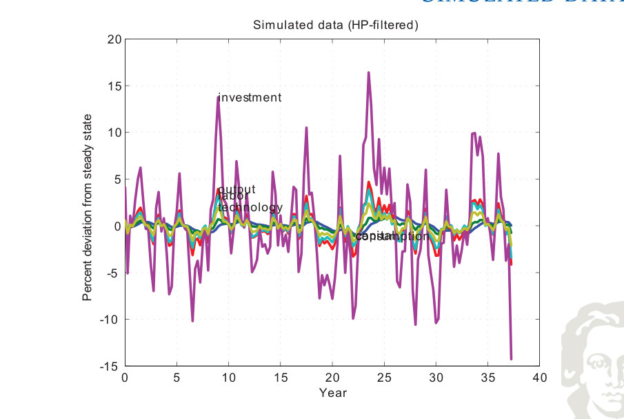
The simulated series are generated by a sequence of technology innovations and then HP-filtered. Their amplitudes and comovement provide model-implied business-cycle moments; unlike a single impulse response, many shocks contribute to the displayed path.
Synthesis
Impulse responses diagnose the propagation mechanism and simulations allow empirical comparison of RBC volatilities and comovements.