Business Cycles Theory and Policy

Come studiareCerca un argomento oppure apri un capitolo dall’indice. I titoli ti portano direttamente alla spiegazione corretta.

2. From traditional macroeconomics to microfoundations

Introduction

The central reason for microfoundations is that a reduced-form rule need not remain stable when policy changes. In a simple Keynesian-cross exercise, consumption responds mechanically to disposable income; in a structural model, the same behavior derives from a household choosing consumption, saving and labor while respecting an intertemporal budget constraint.

The familiar IS–LM framework provides an intuitive description of short-run policy transmission, but its behavioral coefficients and schedules are not a complete theory of individual choice. A change in tax policy or interest-rate expectations may also change the very behavior encoded in those schedules. Microfoundations make those responses explicit by considering preferences, incentives, technologies and information.

The Solow growth model motivates capital accumulation, constant returns to scale and balanced growth. Its saving rate is exogenous, however. An RBC model preserves physical capital accumulation while making consumption, saving and labor supply optimal choices, thereby linking growth-accounting logic to business-cycle propagation.

Integrated theoretical explanation

In a short-run expenditure model, national output is measured by the value of final goods and services produced, while aggregate expenditure is the sum of consumption, investment, government purchases and net exports. For a closed economy, equilibrium in the goods market requires planned spending to equal production. If consumption follows C = c₀ + c₁(Y − T), the marginal propensity to consume c₁ creates a feedback mechanism: additional autonomous demand raises income, some of that income is spent again, and equilibrium output changes by more than the initial demand impulse. This textbook multiplier depends on fixed prices, spare productive capacity and the assumption that the consumption rule does not itself change in response to policy.

The multiplier can be derived directly by collecting income terms. With lump-sum taxes, Y = c₀ + c₁(Y − T) + Ī + G gives (1 − c₁)Y = c₀ − c₁T + Ī + G. Therefore a one-unit increase in government purchases raises equilibrium income by 1/(1 − c₁) units when all other terms are held fixed. If income taxation is proportional, T = tY, the feedback from income to consumption is smaller and the corresponding expression becomes 1/[1 − c₁(1 − t)]. The difference illustrates automatic stabilization: taxes partially offset income movements without the need for a new discretionary fiscal decision.

The IS–LM description adds the interest rate and the money market to the basic goods-market equilibrium. The IS schedule collects combinations of income and the interest rate that are compatible with goods-market equilibrium, taking account of interest-sensitive expenditure. The LM schedule collects combinations that satisfy money demand and money supply at a given price level. A tax increase or fall in spending typically shifts IS to the left, while expansionary monetary policy shifts the LM schedule in the direction associated with lower interest rates at given income. The intersection provides an intuitive joint-equilibrium picture, but changes in expectations, labor supply or saving preferences are not fully explained by the reduced-form curves themselves.

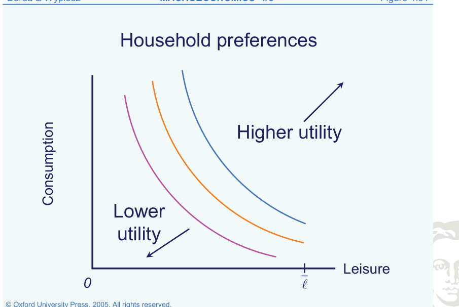
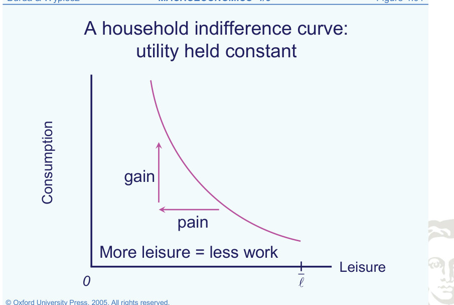
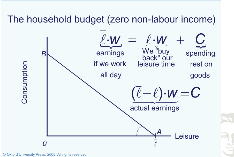
The labor–leisure choice clarifies what is absent from a purely demand-driven representation. A household has a limited time endowment; working more hours produces wage income but leaves less leisure. A consumption–leisure indifference curve describes combinations delivering the same utility, while the budget line translates the wage into the amount of consumption that can be purchased by sacrificing leisure. At an interior optimum, the marginal rate of substitution equals the wage, expressed in appropriate consumption units. A change in taxes on labor income changes this relative price and therefore influences labor supply, which in turn alters aggregate production and the resources available for consumption.

A rise in the real wage has potentially competing effects. Through substitution, leisure becomes more expensive and work becomes more attractive. Through income, a richer household may choose to consume more leisure. Which effect dominates depends on preferences and the context of the wage change. For this reason, a model that assumes fixed labor supply cannot reliably answer every question concerning taxation or productivity. Introducing a utility-based labor supply decision allows the model to distinguish the incentive channel from the income channel and to examine the net outcome in equilibrium with firms' labor demand.

The Solow model supplies the other essential foundation: intertemporal capital accumulation. Output is produced from capital and effective labor, and a fixed fraction of output is invested. The investment rule and capital accumulation identity determine the evolution of productive capacity. When technology and population grow, dividing output and capital by effective labor converts a balanced growth path into a stationary representation. In that normalized economy, investment per effective worker must cover both physical depreciation and the dilution resulting from more effective labor. A stationary capital intensity can therefore coexist with continuing growth in aggregate capital and output.

The saving rule I = sY is useful for understanding transition dynamics but is not an optimal decision derived from household preferences. In a microfounded RBC model, households choose how much to consume and invest after considering future returns and the utility of consumption at different dates. The technology and accumulation equations survive, but the behavioral equation governing saving changes fundamentally. This transition is the intellectual bridge from introductory macroeconomic diagrams to the structural business-cycle model developed later in this volume.

Formal framework and essential relationships

Keynesian-cross benchmark and the fiscal multiplier

Y = c_{0} + c_{1} (Y - T) + \overline{I} + G

Consumption combines autonomous spending c₀ and a fraction c₁ of disposable income; Ī is exogenous planned investment. Goods-market equilibrium requires production Y to match demand.

{\frac{\partial Y}{\partial G} |}_{T f i x e d} = \frac{1}{1 - c_{1}}

An increase in government expenditure becomes income, which induces additional consumption and subsequent production. Under the model’s assumptions, each round is c₁ of the previous one.

\frac{\partial Y}{\partial G} = \frac{1}{1 - c_{1} (1 - t)}, T = t Y

A proportional income tax makes disposable income respond less than one-for-one to production. The tax rate t reduces the multiplier and acts as an automatic stabilizer.

Capital accumulation and balanced growth

Y_{t} = K_{t}^{θ} {(A_{t} L_{t})}^{1 - θ}, K_{t + 1} = (1 - δ) K_{t} + I_{t}

With labor-augmenting technology A and workers L, dividing output and capital by AL produces variables per effective worker, which can converge to constant steady-state values even when aggregates continue to grow.

k_{t + 1} = \frac{(1 - δ) k_{t} + s f (k_{t})}{(1 + μ) (1 + ν)}

This discrete-time effective-worker equation is valid when A and L grow at rates μ and ν and I = sY. It makes the distinction between physical depreciation and dilution by effective-labor growth explicit.

Explanations, derivations and empirical applications

GDP And Demand

A reduced-form relationship gives a useful description of equilibrium under its assumptions. Deriving the underlying choices from household and firm optimization makes it possible to analyze how the relationship responds when policy or incentives change.

National expenditure is composed of consumption, investment, government spending and net exports, so Y = C + I + G + X − IM. In a simple closed economy, net exports disappear and consumption is specified as an increasing linear function of disposable income, C = c₀ + c₁(Y − T). Planned investment is taken as exogenous and the fiscal authorities choose taxes and public purchases. If taxes are proportional to income, T = tY, this creates an automatic stabilizer because a rise in production increases tax revenue and reduces the marginal feedback into private consumption.

Equilibrium On The Goods Market

**Figure 1.** Goods-market equilibrium: planned expenditure and the 45-degree line.

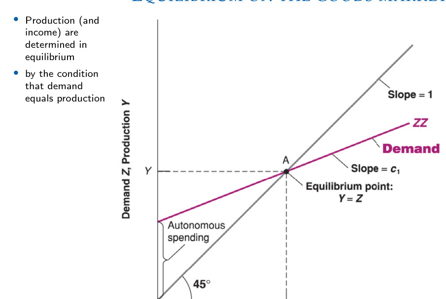
The Keynesian cross determines goods-market equilibrium where planned expenditure intersects the 45-degree line. At the intersection, planned spending equals output. The slope of the expenditure line is the marginal propensity to consume when taxes and investment are fixed.

Government Spending Multiplier

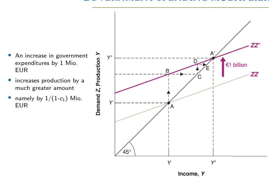
An increase in autonomous government spending shifts planned expenditure upward. Successive rounds of consumption raise equilibrium output by more than the initial expenditure change when the marginal propensity to consume lies between zero and one.

Is-Lm Model

**Figure 3.** IS–LM equilibrium in goods and money markets.

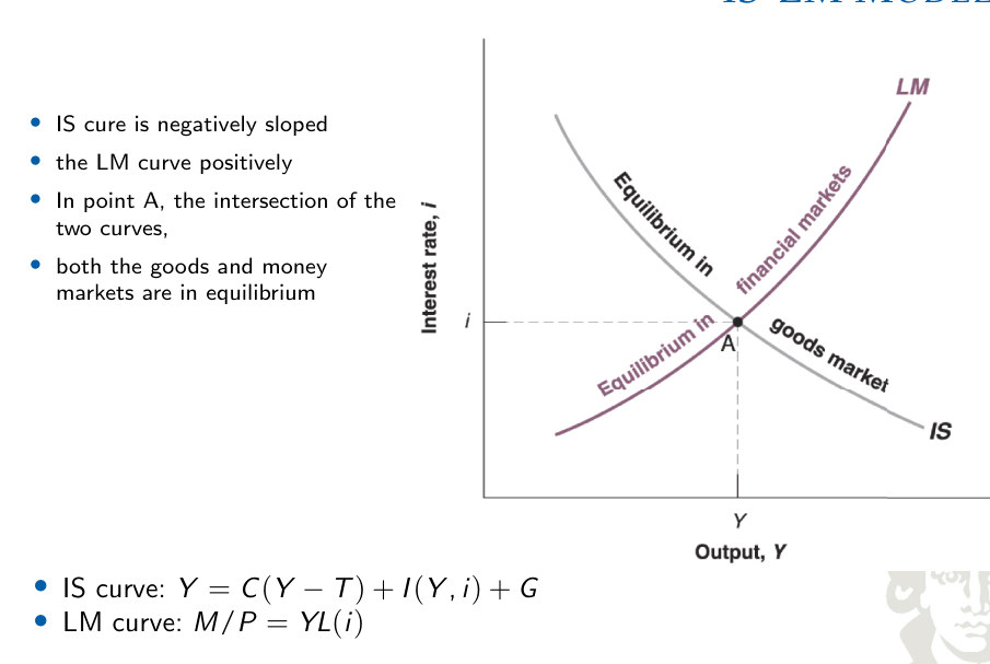
The IS curve represents goods-market equilibrium and slopes downward because higher interest rates reduce interest-sensitive spending. The LM curve represents money-market equilibrium. Their intersection jointly determines output and the interest rate.

Fiscal Policy

**Figure 4.** Tax increase and the leftward shift of the IS curve.

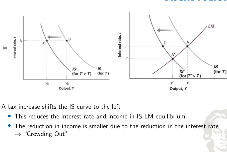
Higher taxes shift the IS curve left by reducing disposable income and consumption. With an unchanged LM curve, both output and the interest rate fall; the lower interest rate partially offsets the contraction by supporting investment.

Monetary Policy

**Figure 5.** Fiscal and monetary responses to a decline in private demand.

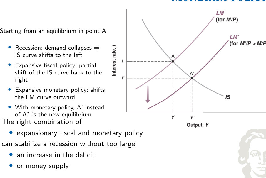
An increase in the real money supply shifts the LM curve outward. The lower equilibrium interest rate supports expenditure and output. Fiscal and monetary adjustments can therefore interact when stabilizing a decline in private demand.

Not All Taxes Are Created Equal

Lump-sum taxes and income taxes do not have identical implications. Changing a fixed tax payment shifts disposable income at every level of production. Changing the marginal income-tax rate also changes the slope of the household’s disposable-income schedule and the strength of the expenditure multiplier. A fuller analysis must additionally account for changes in the relative return to working, which affect the household’s optimal labor–leisure choice.

Consumption and leisure preferences

**Figure 6.** Household indifference map for consumption and leisure; higher curves represent higher utility.

The consumption–leisure indifference curve

**Figure 7.** Consumption–leisure indifference curve and the trade-off from more leisure.

Interpreting household preferences

An indifference curve slopes downward because more leisure must be offset by less consumption to leave utility unchanged. Its slope gives the marginal rate of substitution. Curvature means the willingness to trade leisure for consumption changes across bundles. A higher indifference curve represents greater utility.

The household budget constraint

**Figure 8.** Household budget line linking consumption and leisure at a given real wage.

Choosing an attainable consumption–leisure bundle

**Figure 9.** Attainable and unattainable consumption–leisure bundles and the tangency condition.

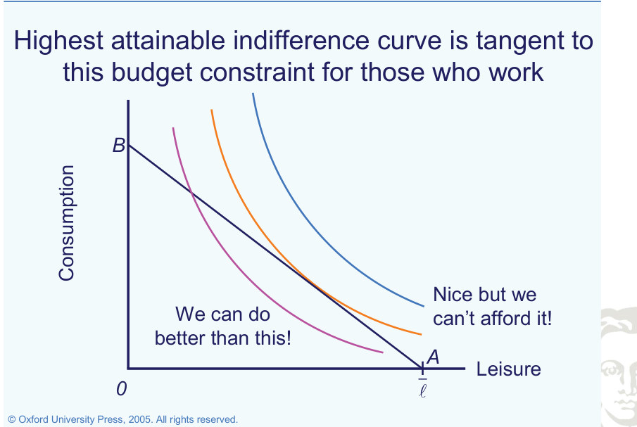
Optimal consumption and leisure

**Figure 10.** Optimal consumption, leisure and working time.

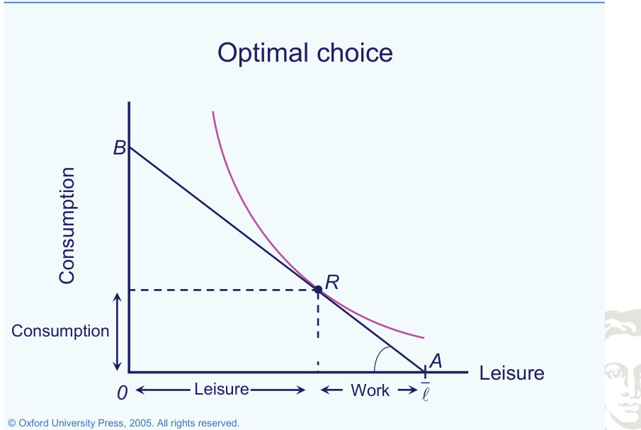
General Equilibrium?

The labor–leisure decision cannot be analyzed in isolation from production. If households prefer more leisure, firms receive less labor input, aggregate output changes and the economy’s feasible consumption possibilities also change. The same feedback operates in reverse when work becomes more attractive. A general-equilibrium analysis incorporates these mutually dependent adjustments rather than shifting one household budget line while leaving all aggregate factor-market conditions unchanged.

Production Function

The Solow production technology combines capital K, labor L and labor-augmenting productivity A, typically through Y = K^θ(AL)^(1−θ). The exponents determine marginal-product elasticities, and their sum of one gives constant returns to scale in the two productive inputs. A rise in A increases effective labor for a given number of workers; capital deepening and technological progress then jointly determine output per worker.

What Do ’Constant Returns To Scale’ Mean?

Constant returns to scale describe a proportional experiment in which every physical input increases by the same factor. With Cobb–Douglas exponents θ and 1 − θ, multiplying both capital and labor by two multiplies output by 2^θ × 2^(1−θ) = 2. This property is different from diminishing marginal returns to increasing capital while labor is held fixed. Both properties can hold simultaneously.

Households

The consumption–leisure trade-off is determined jointly by preferences and the budget opportunity set. Wage and tax changes alter that trade-off and consequently labor supply, output and the feasible aggregate resource allocation.

In the Solow model, households supply labor without an endogenous labor–leisure decision and save a constant fraction s of output. Their investment is therefore Iₜ = sYₜ, while the capital stock changes according to Kₜ₊₁ = (1 − δ)Kₜ + Iₜ. The model is useful for growth accounting and transition dynamics, but the saving decision does not respond optimally to future wages, returns or changes in fiscal policy.

Capital accumulation and timing

Normalizing by effective labor allows a growing aggregate economy to be analyzed using stationary ratios. The balance between saving, investment, depreciation and effective-labor growth determines transitional capital accumulation.

Installed capital becomes available for production after investment. Using the timing convention of the Solow discussion:

K_{t + 1} = (1 - δ) K_{t} + I_{t}, Y_{t + 1} = {(A_{t + 1} L_{t + 1})}^{1 - θ} K_{t + 1}^{θ}

Investment during period t therefore contributes to production in t+1.

Exogenous Growth

Labor supply and labor-augmenting technology grow at externally specified rates. If Aₜ₊₁ = (1 + μ)Aₜ and Lₜ₊₁ = (1 + γ)Lₜ, then effective labor AL grows at the product of those gross rates. This provides the denominator needed for expressing output, capital and investment per unit of effective labor and identifying a stationary representation of a growing economy.

Transformation: Units Of Effective Labor

Normalize variables by effective labor AₜLₜ. With labor-augmenting technology growing at μ and labor at γ:

y_{t} = \frac{Y_{t}}{A_{t} L_{t}}, k_{t} = \frac{K_{t}}{A_{t} L_{t}}, i_{t} = \frac{I_{t}}{A_{t} L_{t}}

y_{t} = k_{t}^{θ}, i_{t} = s y_{t}

(1 + μ) (1 + γ) k_{t + 1} = (1 - δ) k_{t} + s k_{t}^{θ}

\frac{k_{t + 1}}{k_{t}} = \frac{1 - δ + s k_{t}^{θ - 1}}{(1 + μ) (1 + γ)}

Stationary State

A Stationary State is defined as a state where all variables attain constant values.

No population growth, no technological progress µ = γ = 0 (therefore, At = At−1 = A und Lt = Lt−1 = L) and no growth in capital stock (Kt+1 = Kt = K); The capital development equation; Kt+1 = (1 −δ) Kt + It becomes in the Stationary State δK = I; Thus, investments are exactly as high to balance the depreciation of the capital stock K. Investment rule sY = I. A higher savings ratio s enables a higher capital stock, whose depreciation is compensated by investments.

Without population or technological growth, a stationary state satisfies replacement investment equal to depreciation:

δ k = s k^{θ}, k = {(\frac{s}{δ})}^{1 / (1 - θ)}, y = {(\frac{s}{δ})}^{θ / (1 - θ)}

\frac{Y}{L} = A y

Higher saving or lower depreciation raises stationary capital and output per worker.

Steady State

A steady state is the reference allocation in the absence of disturbances. It does not imply that capital can be maintained without investment: gross investment must exactly offset depreciation when aggregate capital is constant.

On a balanced growth path, capital per effective worker remains constant, while aggregate capital and output grow with effective labor. Technical progress raises the effectiveness of labor; it does not mechanically require more workers.

\frac{K_{t + 1}}{K_{t}} = (1 + μ) (1 + γ), \frac{Y_{t}}{K_{t}} = \frac{y}{k}

k = {(\frac{s}{μ + γ + μ γ + δ})}^{1 / (1 - θ)}

y = k^{θ}, \frac{Y_{t}}{L_{t}} = A_{0} {(1 + μ)}^{t} {(\frac{s}{μ + γ + μ γ + δ})}^{θ / (1 - θ)}

The no-growth stationary state is the special case μ = γ = 0. Population growth increases the investment needed to maintain capital per effective worker.

Savings Rate And Consumption

The Golden Rule saving rate maximizes steady-state consumption per effective worker. If the economy accumulates more capital than this benchmark, reducing saving can raise both current consumption and eventual steady-state consumption. In this overaccumulation case, the original path is dynamically inefficient within the model.

Growth Policy

The Golden Rule identifies a consumption-maximizing benchmark for capital accumulation. In a decentralized economy, however, saving arises from private choices rather than a directly imposed aggregate rate. Evaluating policy therefore requires a model that explains how incentives alter household saving.

The intertemporal budget constraint

**Figure 11.** Intertemporal budget line with slope minus the gross interest factor.

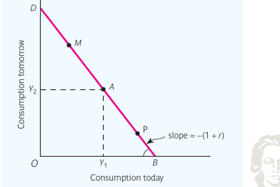
The intertemporal budget line allocates lifetime resources between consumption today and tomorrow. Its slope is minus the gross interest factor, −(1+r): giving up one unit today finances 1+r units tomorrow.

An indifference curve: utility held constant

**Figure 12.** Intertemporal consumption indifference curve.

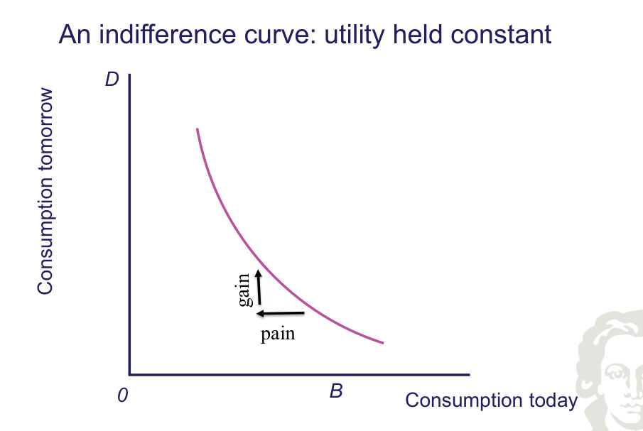
An intertemporal indifference curve joins consumption bundles yielding the same utility. Its downward slope represents willingness to substitute future consumption for current consumption; curvature reflects diminishing marginal utility.

Optimal consumption

**Figure 13.** Optimal intertemporal consumption at a budget-line tangency.

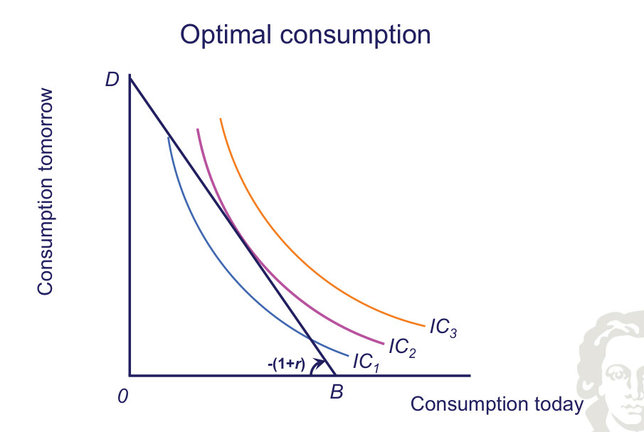
The optimal intertemporal consumption allocation is the tangency between the highest attainable indifference curve and the lifetime budget line. At an interior solution, the intertemporal marginal rate of substitution equals the gross interest factor.

Optimal consumption: borrowing

**Figure 14.** Borrower consumption allocation and future repayment.

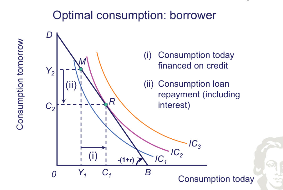
A borrower consumes more than current income and repays principal plus interest from future income. The budget line and preferences determine the optimal amount borrowed.

Optimal consumption: lending

**Figure 15.** Lender consumption allocation and future interest income.

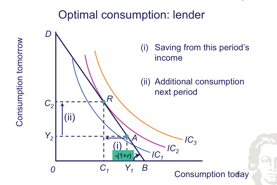
A lender consumes less than current income and carries saving forward with interest. The optimum balances the utility cost of lower current consumption against the utility benefit of higher future consumption.

Tools Of The Trade

The RBC model emphasizes optimizing intertemporal choices, capital accumulation and real productivity shocks. New Keynesian models retain dynamic optimization while adding nominal price-setting frictions, making monetary-policy transmission and stabilization central to the analysis.

Synthesis

Behavioral equations derived from intertemporal optimizing agents can respond to changes in incentives, which is essential for structural policy analysis.

Torna all’inizio ↑