
4. The Real Business Cycle model: the firm
Introduction
The RBC economy features optimizing households and firms trading output, labor services and capital services in competitive markets. Firms hire inputs after observing available technology and choose quantities until each factor's marginal product equals its competitive rental price.
The standard production function has Cobb–Douglas form. Its exponent on capital determines the capital income share, and its exponent on labor determines the labor income share when markets are competitive and production has constant returns to scale. Because current output uses the predetermined capital stock inherited from the preceding period, new investment first affects productive capacity in a later period.
Productivity changes are represented by an autoregressive process. Persistence matters: a temporary technological innovation can influence a sequence of future periods, causing households to adjust consumption and investment immediately in anticipation of the future.
Integrated theoretical explanation
The competitive RBC economy consists of a representative household and a representative firm. Firms transform labor services and installed capital services into a final good. Households supply labor, own capital and receive factor income and any distributed profits; they allocate the final good between consumption and investment. In the benchmark closed economy there is only one produced good and no government sector, so aggregate output must equal the resources absorbed by consumption and investment. These simplifying assumptions make the intertemporal mechanism transparent and allow every market-clearing condition to be written precisely.
The firm produces according to yₜ = zₜ kₜ₋₁^α nₜ^(1−α). The variable zₜ is total factor productivity, nₜ is current labor input, and kₜ₋₁ is capital already installed at the start of period t. The exponent α lies between zero and one. Since the exponents add up to one, increasing capital and labor by the same proportion increases output by that proportion; this is constant returns to scale. It does not mean that output grows linearly in one input when the other is held fixed: diminishing marginal productivity with respect to each single input remains present.
A competitive firm takes the real wage wₜ and capital rental rate rₜ as given and maximizes profit, yₜ − wₜnₜ − rₜkₜ₋₁. Differentiating output with respect to labor gives the marginal product of labor (1 − α)yₜ/nₜ, so the optimal labor demand condition is wₜ = (1 − α)yₜ/nₜ. Differentiating with respect to capital gives αyₜ/kₜ₋₁, so rₜ = αyₜ/kₜ₋₁. These are marginal-product pricing conditions, not identities that hold under arbitrary market structure. Under perfect competition and constant returns to scale, payments to labor and capital exhaust output in the benchmark.
The timing convention is economically significant. Capital kₜ₋₁ can be used immediately because it already exists when the period begins, whereas investment selected during period t only contributes to installed capital kₜ and thus to subsequent production. Labor can respond during the current period once the wage and productivity are observed. Confusing kₜ with kₜ₋₁ would alter the model's state structure and can produce incorrect impulse responses, because it would permit today's investment to be used prematurely as today's productive capital.
The productivity state has a stochastic law of motion ln zₜ = ρ ln zₜ₋₁ + uₜ. The innovation uₜ is the newly arriving surprise, while zₜ incorporates the persistent effects of previous surprises. If 0 < ρ < 1, a one-time positive innovation raises current productivity and then decays in expectation at rate ρ. A ρ near one implies a long-lived disturbance; a ρ near zero implies rapid reversion to the normalized steady-state level. Knowing the transition rule and the distribution of innovations enables households to form rational expectations about future productivity.
A favorable technology disturbance shifts the production function outward, raising output for given inputs and increasing the marginal products of capital and labor. Its general-equilibrium effect is more complicated than this direct production shift because higher wages and returns induce households to change hours, consumption and investment. The firm block supplies the demand side of those factor markets, but it does not determine employment or capital accumulation by itself. Those outcomes emerge only after combining factor demand with optimal household decisions, resource feasibility and the shock process.
Formal framework and essential relationships
Current output depends on contemporaneous labor, inherited capital and productivity. The no-growth normalization sets labor-augmenting trend A to one; it does not eliminate stochastic productivity z.
Firms take real wage w and capital rental rate r as given. The decision is static once z and prices are known, although capital is predetermined at the aggregate level.
Under competitive factor demand, each price equals its marginal product. Consequently, wage income is (1−α) of production and gross capital rental income is α of production.
The shock innovation u is not identical to total technology z: z includes the accumulated effects of persistent past innovations. When 0 < ρ < 1, the expected effect decays geometrically.
Explanations, derivations and empirical applications
The economy and its market structure
The competitive conditions and the timing of installed capital jointly determine factor demand. Current technology affects marginal products immediately, whereas investment changes productive capacity only after the installation period.
Productivity disturbances and production
Real Business Cycle Model
A standard RBC economy combines optimizing households and firms with perfectly competitive markets. Households determine consumption, investment and labor supply, while firms demand inherited capital and contemporaneous labor to maximize profit. Aggregate productivity evolves stochastically. The objective is to determine whether productivity innovations transmitted through these optimizing decisions can account for the main observed patterns of aggregate fluctuations.
How the RBC model extends the Solow framework
The RBC framework makes productivity stochastic and allows households to choose consumption, saving and labor supply. The basic Solow model instead imposes a saving rate and labor path.
Goods
Three markets connect households and firms: a final good used for consumption or investment, labor services supplied by households, and capital services supplied by households. Households receive factor income from firms and use it to finance consumption and accumulation. Firms combine the services into output, and the quantities supplied and demanded must coincide at equilibrium prices.
Market Structure
All three markets are perfectly competitive in the benchmark. Individual agents treat the real wage, capital rental rate and final-good price as given, and no firm possesses market power over factor prices or output. This assumption yields marginal-product conditions that allow factor prices to be eliminated from the equilibrium system. It is a modelling simplification whose usefulness depends on the question under investigation.
Information Structure
The period’s productivity state is known when labor and production decisions are made, while the next innovation remains uncertain. Installed capital is inherited from the previous period. Rational expectations require households and firms to use the stochastic structure of the model consistently when anticipating future prices, productivity and returns. Their forecasts need not be perfect, but they must reflect the information and probabilities specified by the model.
Model Environment
The benchmark economy is closed, contains a representative firm and household, and has a single final output good. Firms rent capital and hire labor, while households own the productive assets, supply time and choose consumption and saving. The exclusion of government demand, external trade and nominal rigidities makes the central RBC propagation mechanism easier to trace, but it also restricts which policy questions the model can answer.
Elements Of A Competitive Equilibrium
Households own time, capital and firms; receive wages, capital rental income and profits; and choose labor, investment and consumption to maximize utility. Firms hire labor and capital to maximize profit. Market clearing determines wages and rental rates and requires the goods allocation to satisfy the resource constraint.
Stochastic Production
Production combines a labor-augmenting trend Aₜ and stochastic total factor productivity zₜ.
What Is An AR(1)-Process?
An AR(1) process relates the current value to one lag and a new innovation. The innovation has zero mean, constant variance and is independent across dates. The coefficient ρ measures persistence; covariance stationarity requires |ρ| < 1.
Example AR(1)-Process
Let x₋₁ = 0, set u₀ = 1 and all later innovations to zero. Then:
With ρ = 0.9 the response in period 4 is 0.6561. For |ρ| < 1 it decays to zero.
Fit to text
Scroll horizontally to inspect the labels and values.
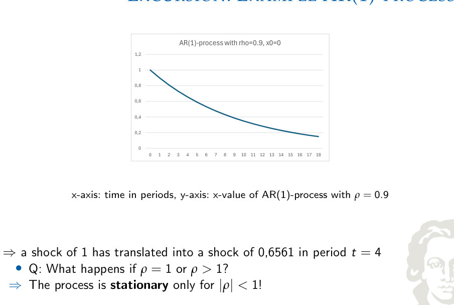
Effect Of Productivity Shocks
An AR(1) process describes persistence with a first-order lag: today's state depends on yesterday's state plus a new innovation. If the persistence parameter lies between zero and one, a positive surprise gradually fades; if it is near one, the disturbance remains influential for many periods. Rational expectations use the probability distribution implied by the model and available information, not perfect foresight.
The stationary mean of log productivity is zero. Its deterministic steady-state level is therefore one. A zero mean of log productivity does not, in general, imply that the stochastic mean of productivity itself equals one.
At fixed labor and inherited capital, zₜ above one raises output relative to the deterministic benchmark; zₜ below one lowers it. This comparison is a level effect at given inputs, not a claim about the unconditional mean of output.
Productivity And RBC
The model describes propagation—the sequence of changes in output, hours, consumption and investment following a productivity innovation—and amplification, the size of those changes relative to the initial shock. Its solution consists of dynamic decision rules and impulse response functions.
Technology: Simplification
Set the labor-augmenting trend Aₜ to one to focus on stationary business-cycle deviations.
Constant Returns To Scale?
Scaling capital and labor by a positive common factor q scales output by q:
The technology has constant returns to scale. Competitive factor payments therefore exhaust output.
Profit Maximization By The Firm
The wage and rental conditions are found by differentiating the profit objective separately with respect to labor and capital. Factor shares exhaust output only because the Cobb–Douglas technology has constant returns and inputs receive their competitive marginal products.
Competitive firms take wages and capital rental rates as given. They choose the input quantities that maximize output value less labor and capital costs.
At given factor prices, substitute the production constraint into profits:
An individual firm chooses rented input services; the aggregate stock available for rental is predetermined.
These marginal-product conditions imply rₜkₜ₋₁ + wₜnₜ = yₜ. Productivity affects wages and rental income through both technology and the equilibrium allocation.
Synthesis
Competition and Cobb–Douglas production connect wages and capital returns to marginal products; productivity is an exogenous persistent state.