Business Cycles Theory and Policy

Introduction

Before asking whether a model explains recessions and expansions, we must decide what counts as a cyclical deviation in the data. Raw output levels mix long-run growth with shorter-run fluctuations. Trend extraction is therefore a substantive modelling and measurement choice, not a cosmetic correction.

The empirical analysis uses linear trends, Hodrick–Prescott filtering and band-pass/high-pass ideas, and shows the transformation of consumption, investment, government expenditure and international flows across different economies. A model should be evaluated using compatible definitions, frequencies, seasonal adjustments and filtering rules.

Two sets of moments matter. Kaldor's facts characterize balanced growth over long horizons: labor productivity and capital per worker tend to grow, while the return to capital, the capital–output ratio and factor income shares are comparatively stable. Business-cycle moments characterize volatility, comovement and timing: investment is typically far more volatile than output, while consumption fluctuates less and several aggregates move procyclically.

Integrated theoretical explanation

Observed macroeconomic series combine several time scales. Long-run growth reflects changes in technology, labor and capital; the medium-run component contains recurring expansions and contractions; and very short-run variation can be seasonal or irregular. These are analytic distinctions, not three separately observable objects. An increase in real GDP from one quarter to the next may occur even when output is below its estimated trend, because positive growth and a negative output gap are different statements. Measuring the business cycle therefore requires an explicit choice about the underlying series and the meaning of its trend.

The contrast between nominal output and real output is fundamental. A nominal expenditure series can increase because of higher prices, greater quantities or both; a real series aims to remove the price-level component. Per-capita or per-worker measures answer still different questions, because they adjust for changes in population or labor input. Taking logarithms can make trends more comparable across time and allows log deviations to be interpreted approximately as proportional departures. Before computing a standard deviation or correlation, the sample period, deflator, treatment of seasonality, transformation and measurement units should all be consistent across series.

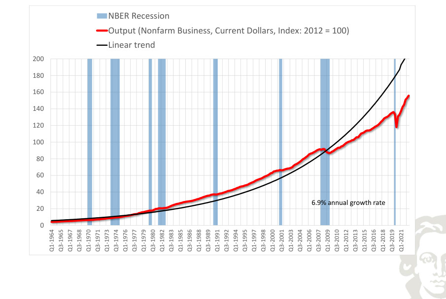
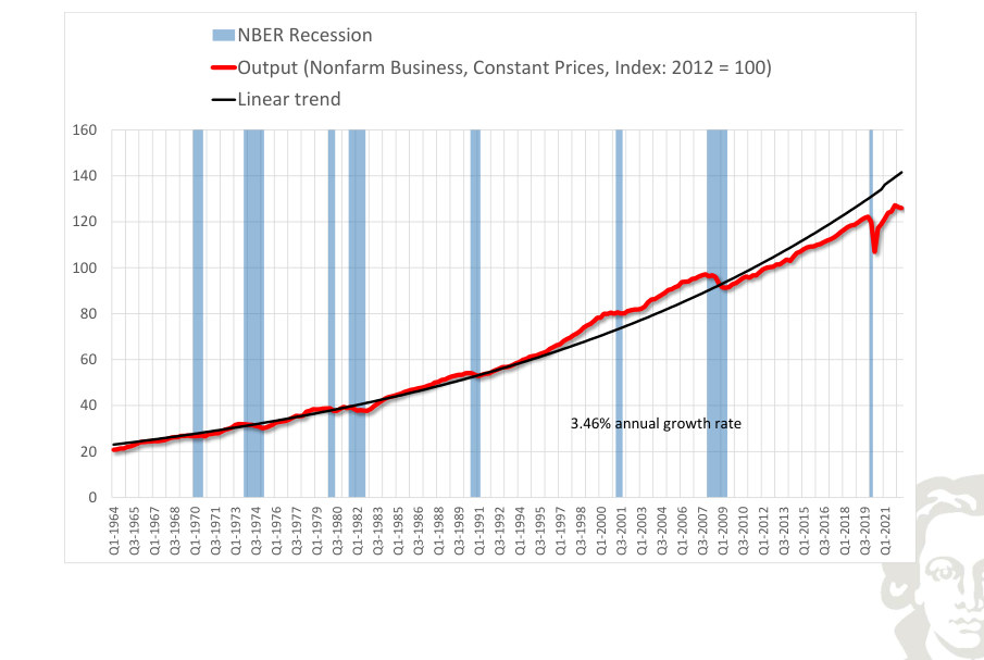
A deterministic linear trend in log output describes a constant average proportional growth rate. Subtracting it yields an output cycle measured relative to this preselected path. Its simplicity is an advantage, but the method is potentially misleading if trend growth changes over time. Conversely, allowing the trend to move too easily can remove genuine cyclical variation. A mechanical trend estimate is consequently not a neutral fact about the data: it embodies a view about which movements are persistent enough to count as growth rather than business cycles.

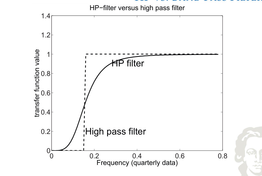
The Hodrick–Prescott filter chooses a smooth trend by minimizing the sum of squared deviations from the observations plus a penalty on variation in the trend's slope. A higher smoothing parameter makes the estimated trend less flexible. The cycle is the difference between the original series and this trend. The procedure is convenient because it produces an operational definition without specifying a full structural model, but it is sensitive to the smoothing choice and to the sample end points. Since the current end of a time series has no future observations available to anchor its trend, revisions can be especially large there.

Band-pass filters address frequency ranges more explicitly. Rather than isolating all residual variation after a smooth trend is removed, a band-pass approach attempts to retain fluctuations with durations within a prescribed interval. This emphasizes that the business cycle is partly defined by periodicity. Filters need not give identical turning points or amplitudes, even when applied to the same national-accounts data. Empirical model comparisons are strongest when the simulated and observed series are subjected to the same transformation instead of comparing unfiltered model deviations with filtered data.

The long-run stylized facts associated with Nicholas Kaldor describe the broad shape of economic growth. Output per worker and capital per worker tend to rise over time, while the capital–output ratio, the rate of return on capital and labor and capital income shares are comparatively stable in a balanced-growth characterization. The Solow model with suitable production technology can reconcile these facts: labor-augmenting technical progress raises productivity, while capital deepening keeps the ratio of capital to effective labor near its stationary value. These properties concern a long-horizon trend and should not be confused with the amplitude of quarterly cyclical fluctuations.

Business-cycle moments instead describe how variables move around their trends. Standard deviation measures typical cyclical dispersion; relative standard deviation divides this measure by that of output. A positive contemporaneous correlation with output indicates procyclical comovement, while a negative one indicates countercyclical movement. Lead–lag correlations examine the timing of a variable's fluctuations relative to output. The broad empirical pattern motivating the RBC benchmark is that consumption is relatively smooth, investment is considerably more volatile than output, and hours worked and many private spending aggregates are procyclical. Capital stock itself usually adjusts much more gradually than gross investment.

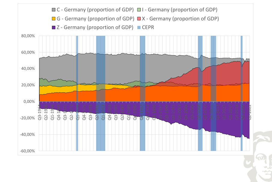
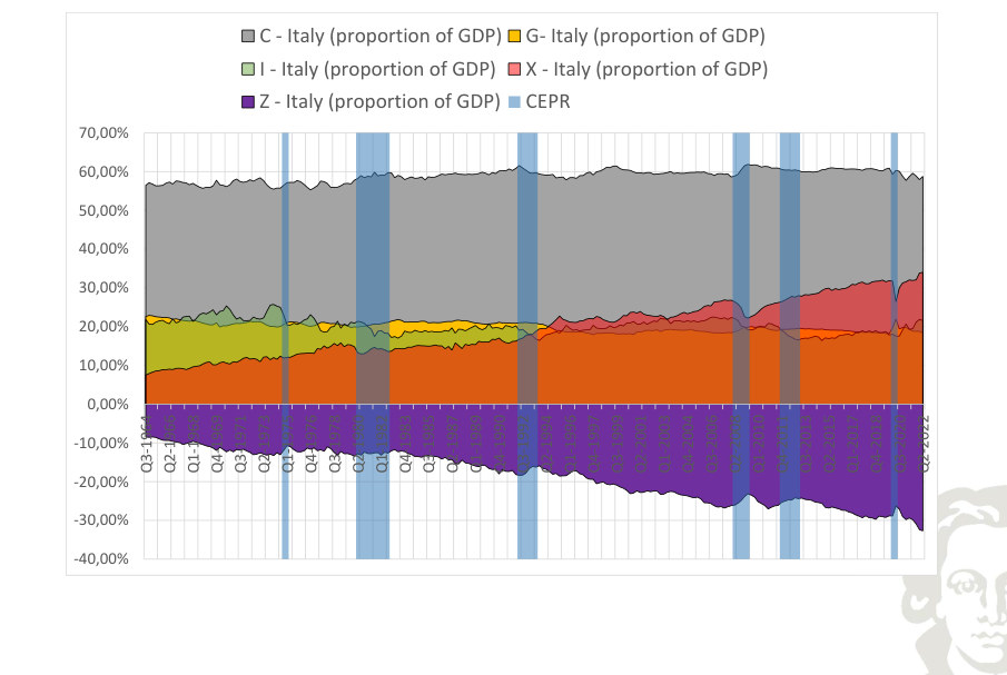
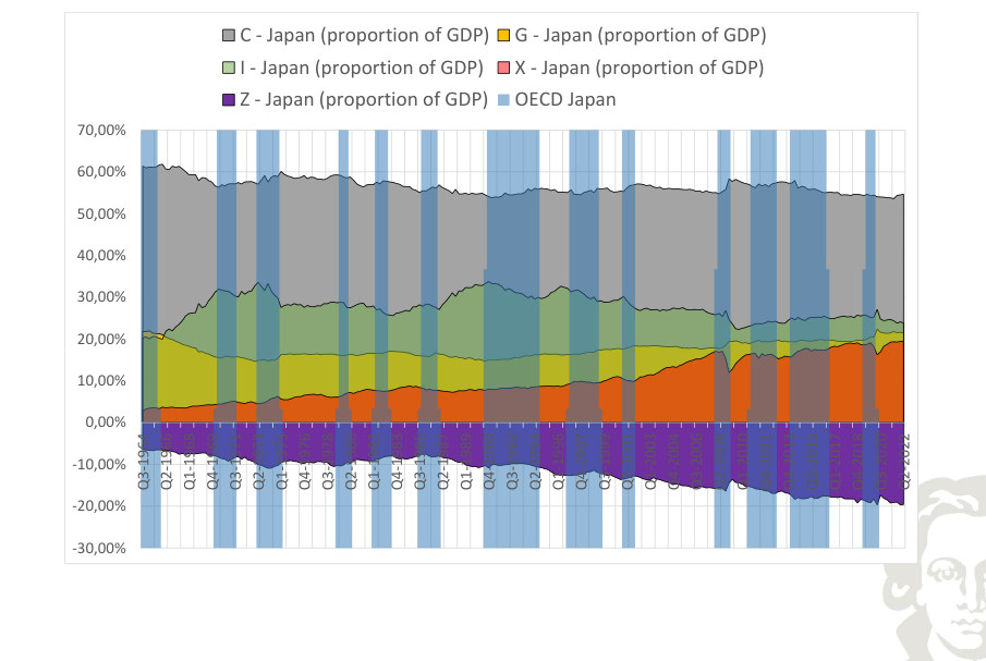
The country and component comparisons matter because no single historical plot can establish a universal regularity. A recession can be global or concentrated in one economy; import and export series reflect external demand and national-accounting differences; and public expenditure need not follow the same cyclical pattern as private investment. When looking at output, consumption, investment, public demand or external flows across different geographic samples, the purpose is to determine which properties are sufficiently persistent to serve as meaningful quantitative targets. The RBC model should be judged on a defined collection of moments, not on whether one chart happens to look similar.

Formal framework and essential relationships

Three concepts of cyclical data

log Y_{t} = {trend}_{t} + {cycle}_{t}

On the log scale, a deviation can be read approximately as a percentage above or below trend. Trends and cycles are measured constructs, not directly observed separate quantities.

min_{{τ_{t}}} {\sum_{t} {(y_{t} - τ_{t})}^{2} + λ \sum_{t} {[(τ_{t + 1} - τ_{t}) - (τ_{t} - τ_{t - 1})]}^{2}}

The Hodrick–Prescott filter selects the trend τ to trade off fidelity to the observed series against smoothness of its growth. The parameter λ penalizes changes in the trend slope.

Kaldor facts and cyclical moments must not be confused

Object	Long-run / business-cycle role	Relevant measure
Output per worker	Growth regularity	Y/L
Capital intensity	Growth regularity	K/L
Factor income shares	Growth regularity	wL/Y and rK/Y
Relative volatility	Business-cycle dispersion	sd(xᶜ)/sd(Yᶜ)
Contemporaneous correlation	Business-cycle comovement	corr(xᶜ,Yᶜ)
Lead–lag correlation	Timing	corr(xₜ₊ⱼᶜ,Yₜᶜ)

Empirical business-cycle moments

Series	Standard deviation	Relative to GDP
GDP	0.016	1.0
Non-durable consumption	0.014	0.906
Investment	0.064	4.134
Capital	0.007	0.446
Total hours	0.02	1.315
Employment	0.014	0.879
Average hours	0.009	0.592
Labor productivity	0.01	0.644
TFP	0.012	0.774

These empirical moments refer to the defined series and detrending transformations. The quantitative model should be evaluated using moments computed on the same basis.

Explanations, derivations and empirical applications

What Are Business Cycles?

Business-cycle statistics summarize recurring comovement and variability in macroeconomic data. Results depend on how the raw series are transformed and which frequency range is taken to represent the cycle.

Business cycles are broad fluctuations in aggregate economic activity rather than movements in a single sector. The classic characterization of Burns and Mitchell distinguishes expansions spread across many activities from similarly widespread contractions, revivals and subsequent expansions. Their duration is not fixed: historical cycles have varied considerably in length. Their defining characteristics include comovement, persistence and a recognizable sequence of phases.

Why The Cycle?

Studying aggregate fluctuations requires tracking many interrelated variables rather than treating output alone as the cycle. Consumption, investment, labor inputs, productivity and other indicators can have different amplitudes and timing. In the spirit of Sims’s argument for confronting macroeconomic theory with reality, statistical models and carefully transformed observations supply a common arena in which competing mechanisms can be quantitatively evaluated.

Decomposing observed macroeconomic data

A common decomposition expresses an observed economic series as a trend component plus a cyclical deviation. The appropriate trend may be suggested by theory, as in the balanced growth path of the neoclassical growth model, but not every variable has a constant trend after simple normalization. Hours per worker, participation and population-related measures may exhibit their own long-run movements. Therefore, the chosen decomposition must be justified separately for the variables being studied.

NBER Recession Output (Nonfarm Business, Current Dollars, Index: 2012 = 100)

**Figure 16.** Nominal nonfarm-business output index with NBER recession shading.

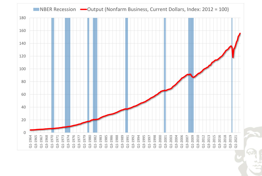
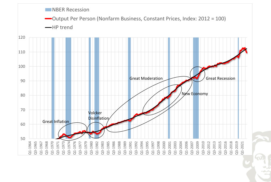
Separating a stochastic cycle from an estimated trend requires selecting an observed series, a trend specification and a smoothing convention. Changes in the trend estimator alter the measured cycle; recession bands provide historical context rather than mechanically defining the cyclical component.

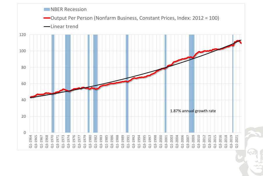
Linear Trend (In Logs)

A linear trend in log output imposes a constant average growth rate. The cyclical component is the difference between observed log output and its estimated trend:

log Y_{t}^{c y c l e} = log Y_{t} - log Y_{t}^{t r e n d}

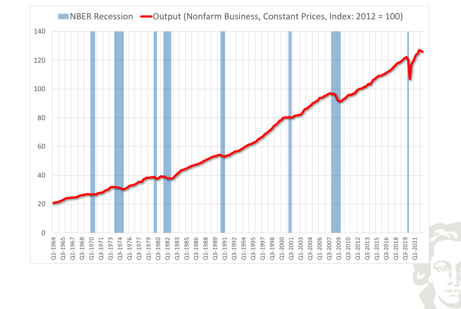
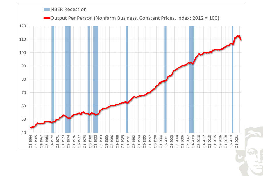
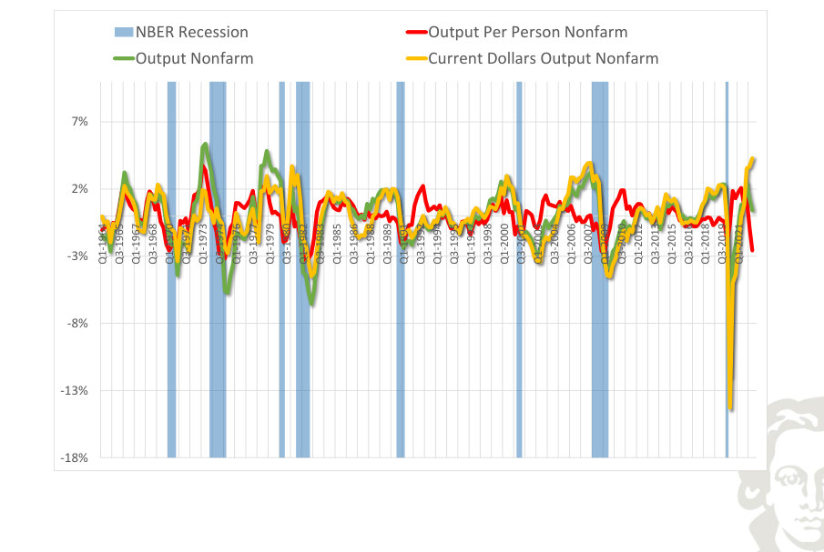
Using real rather than nominal output removes price-level changes, but a fixed trend can still miss changes in growth. Statistical filters allow a time-varying trend.

NBER Recession

NBER Recession Output (Nonfarm Business, Constant Prices, Index: 2012 = 100)

NBER Recession

**Figure 19.** Real nonfarm-business output and fitted trend.

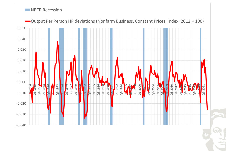
NBER Recession Deviations from trend

**Figure 20.** Output deviations from a deterministic trend.

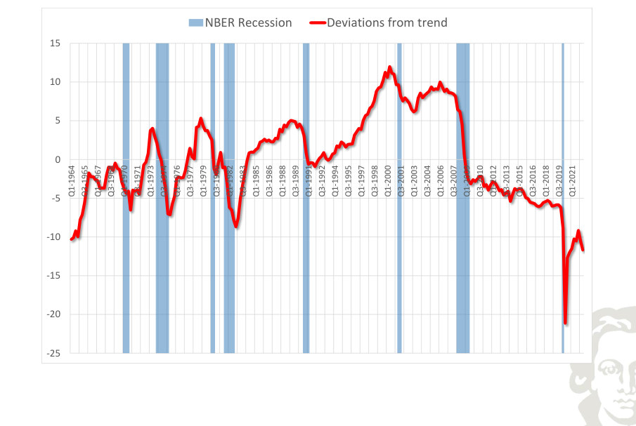
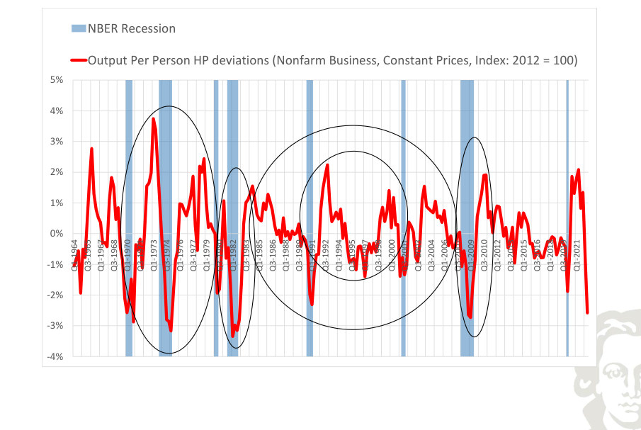
Detrended macroeconomic activity for the selected economy highlights movements above and below the estimated long-run path. The horizontal zero line is a normalization relative to the chosen filter, not a literal condition of zero production. Compare the timing and amplitude of these fluctuations with the corresponding output series.

NBER Recession

**Figure 21.** Real nonfarm-business output per person.

**Figure 22.** Real output per person and fitted linear trend.

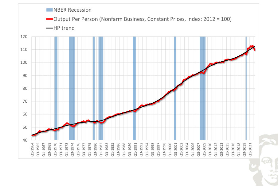
A Statistical Method: Hodrick-Prescott Filter

Separate the observed series into trend and cycle. The HP filter chooses the trend to minimize:

min_{{τ_{t}}_{t = 1}^{T}} {\sum_{t = 1}^{T} {(y_{t} - τ_{t})}^{2} + λ \sum_{t = 2}^{T - 1} {[(τ_{t + 1} - τ_{t}) - (τ_{t} - τ_{t - 1})]}^{2}}

A larger λ penalizes changes in trend growth more heavily. At λ = 0 the trend follows the data exactly; as λ grows without bound, the fitted trend approaches a straight line.

NBER Recession

**Figure 23.** Real output per person and its HP-filter trend.

**Figure 24.** HP trend with selected historical economic episodes marked.

**Figure 25.** HP-filtered cyclical deviations of output per person.

**Figure 26.** Cyclical output deviations with historical phases highlighted.

NBER Recession Output Per Person Nonfarm

**Figure 27.** Comparison of cyclical output measures under alternative normalizations.

HP Vs. Band Pass Filter

**Figure 28.** Transfer functions of the HP filter and an ideal high-pass filter.

Stylized Macro Facts

National expenditure and its transformations:

Y_{t} = C_{t} + G_{t} + I_{t} + X_{t} - I M_{t}, Y_{t} = Y_{t}^{t r e n d} + Y_{t}^{c y c l e}

g_{Y, t} = \frac{Y_{t} - Y_{t - 1}}{Y_{t - 1}}

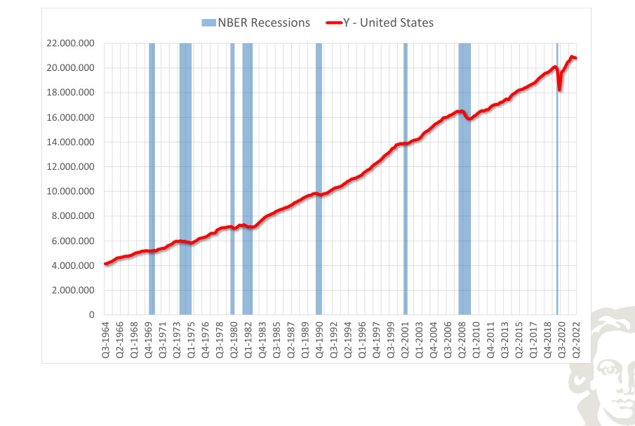
The growth formula compares consecutive observations. The time interval and any annualization must be specified. Source for the country series: OECD.

USA · country series

NBER Recessions Y - United States

**Figure 29.** United States: output, level, with recession shading.

NBER Recessions Y - United States (Annual Growth)

**Figure 30.** United States: output, growth rate, with recession shading.

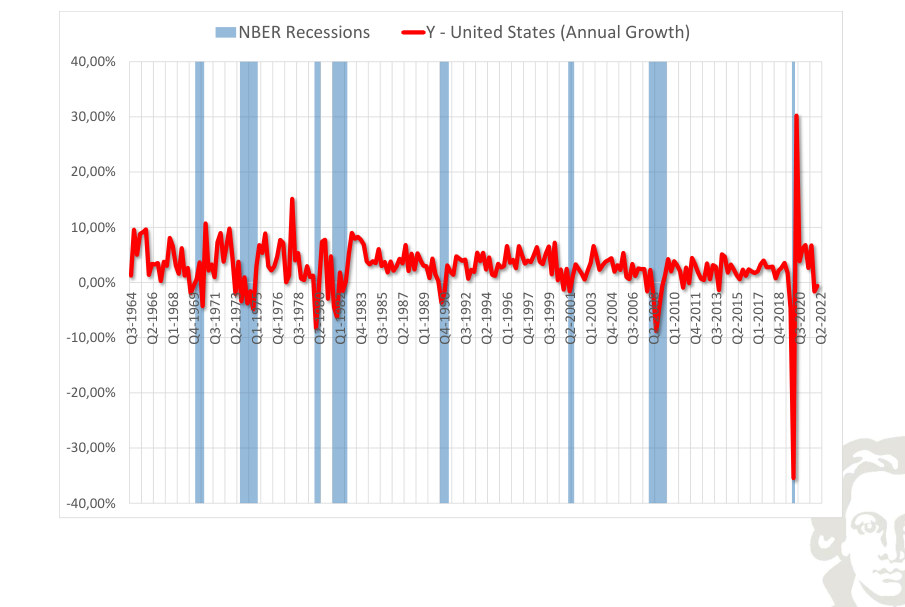
The plotted growth rate of real output for the United States measures the change in activity under the frequency and rate convention of the series. Negative growth and below-trend growth are different concepts; comparing them helps identify contractions without assuming that every slowing constitutes a recession.

NBER Recessions Y - United States (Annual Trend Growth)

**Figure 31.** United States: output, smoothed trend growth, with recession shading.

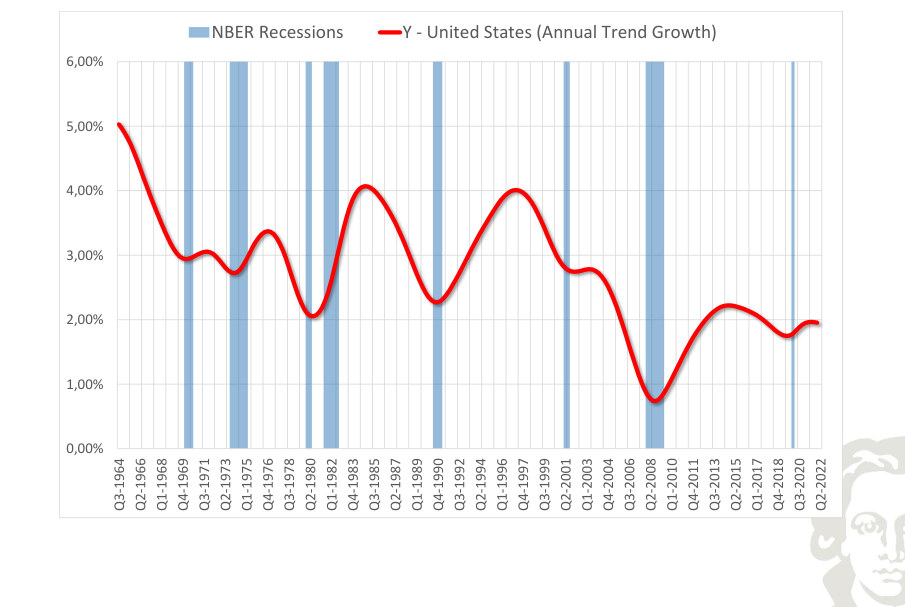
The smoothed growth path of real output in the United States describes the slower-moving change in the rate of expansion. It should not be equated with the cyclical component: the trend-growth series may slow even when the level of activity continues to rise.

NBER Recessions Y - United States (Deviations from Trend)

**Figure 32.** United States: output, deviation from trend, with recession shading.

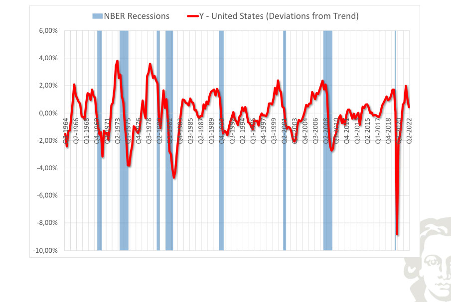
Detrended real output for the United States highlights movements above and below the estimated long-run path. The horizontal zero line is a normalization relative to the chosen filter, not a literal condition of zero production. Compare the timing and amplitude of these fluctuations with the corresponding output series.

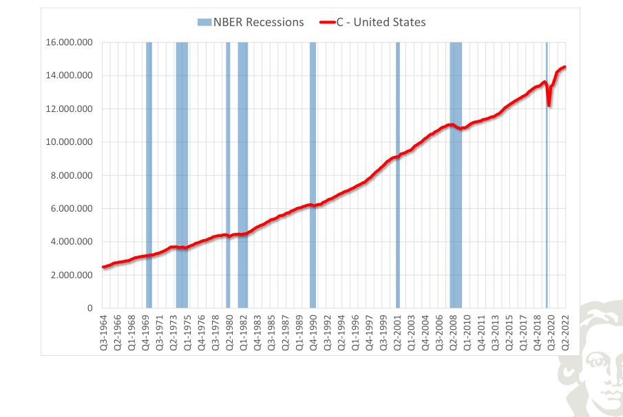
NBER Recessions C - United States

**Figure 33.** United States: consumption, level, with recession shading.

NBER Recessions C - United States (Annual Growth)

**Figure 34.** United States: consumption, growth rate, with recession shading.

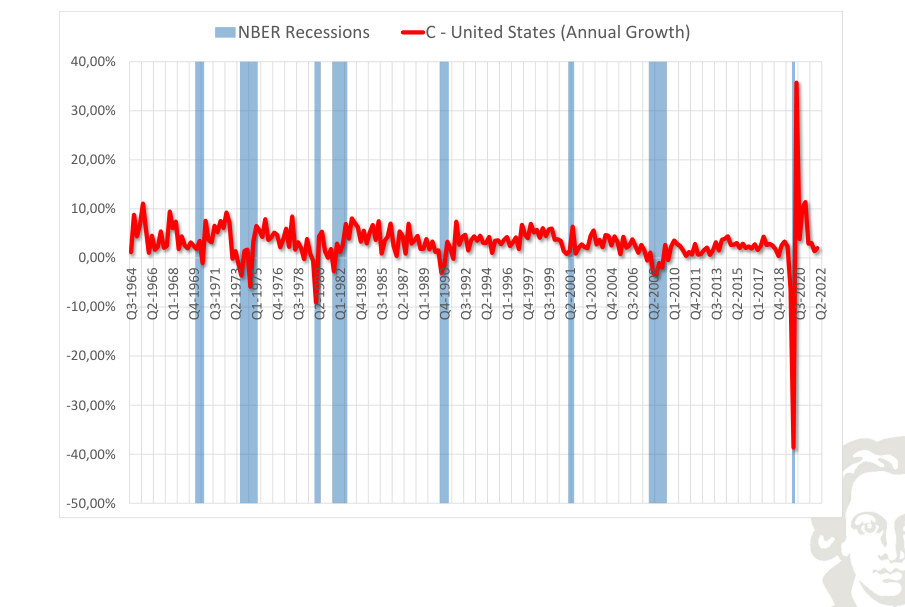
The plotted growth rate of consumption for the United States measures the change in activity under the frequency and rate convention of the series. Negative growth and below-trend growth are different concepts; comparing them helps identify contractions without assuming that every slowing constitutes a recession.

NBER Recessions C - United States (Annual Trend Growth)

**Figure 35.** United States: consumption, smoothed trend growth, with recession shading.

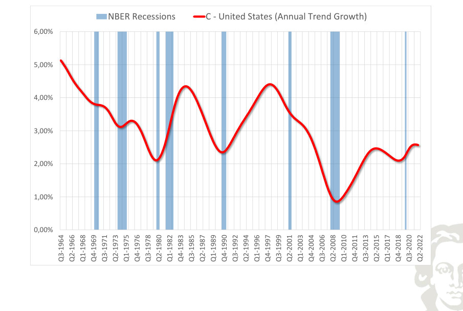
The smoothed growth path of consumption in the United States describes the slower-moving change in the rate of expansion. It should not be equated with the cyclical component: the trend-growth series may slow even when the level of activity continues to rise.

NBER Recessions C - United States (Deviations from Trend)

**Figure 36.** United States: consumption, deviation from trend, with recession shading.

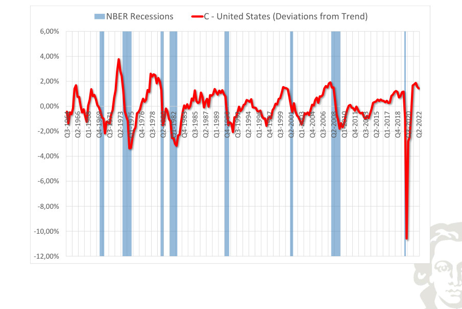
Detrended consumption for the United States highlights movements above and below the estimated long-run path. The horizontal zero line is a normalization relative to the chosen filter, not a literal condition of zero production. Compare the timing and amplitude of these fluctuations with the corresponding output series.

NBER Recessions I - United States

**Figure 37.** United States: investment, level, with recession shading.

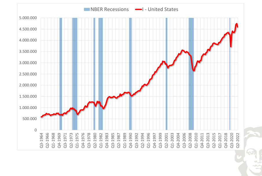
NBER Recessions I - United States (Annual Growth)

**Figure 38.** United States: investment, growth rate, with recession shading.

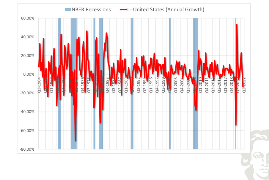
The plotted growth rate of investment for the United States measures the change in activity under the frequency and rate convention of the series. Negative growth and below-trend growth are different concepts; comparing them helps identify contractions without assuming that every slowing constitutes a recession.

NBER Recessions I - United States (Annual Trend Growth)

**Figure 39.** United States: investment, smoothed trend growth, with recession shading.

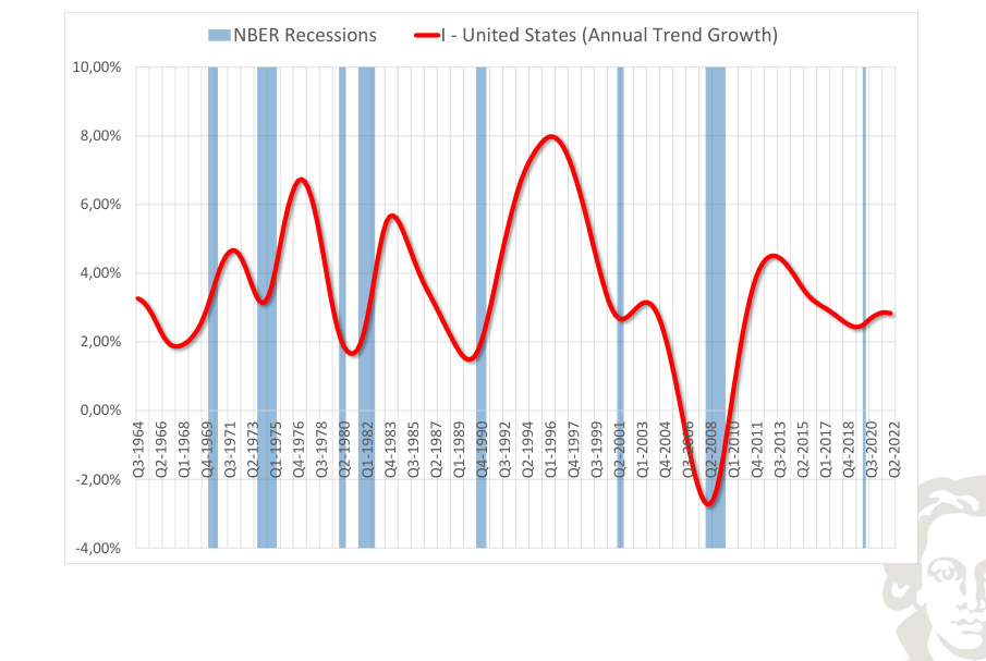
The smoothed growth path of investment in the United States describes the slower-moving change in the rate of expansion. It should not be equated with the cyclical component: the trend-growth series may slow even when the level of activity continues to rise.

NBER Recessions I - United States (Deviations from Trend)

**Figure 40.** United States: investment, deviation from trend, with recession shading.

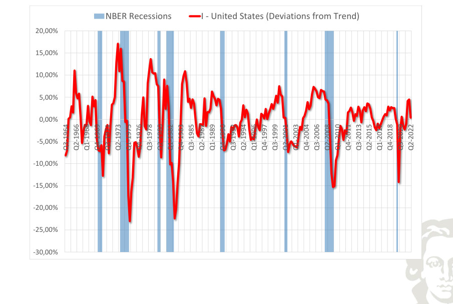
Detrended investment for the United States highlights movements above and below the estimated long-run path. The horizontal zero line is a normalization relative to the chosen filter, not a literal condition of zero production. Compare the timing and amplitude of these fluctuations with the corresponding output series.

NBER Recessions G - United States

**Figure 41.** United States: government expenditure, level, with recession shading.

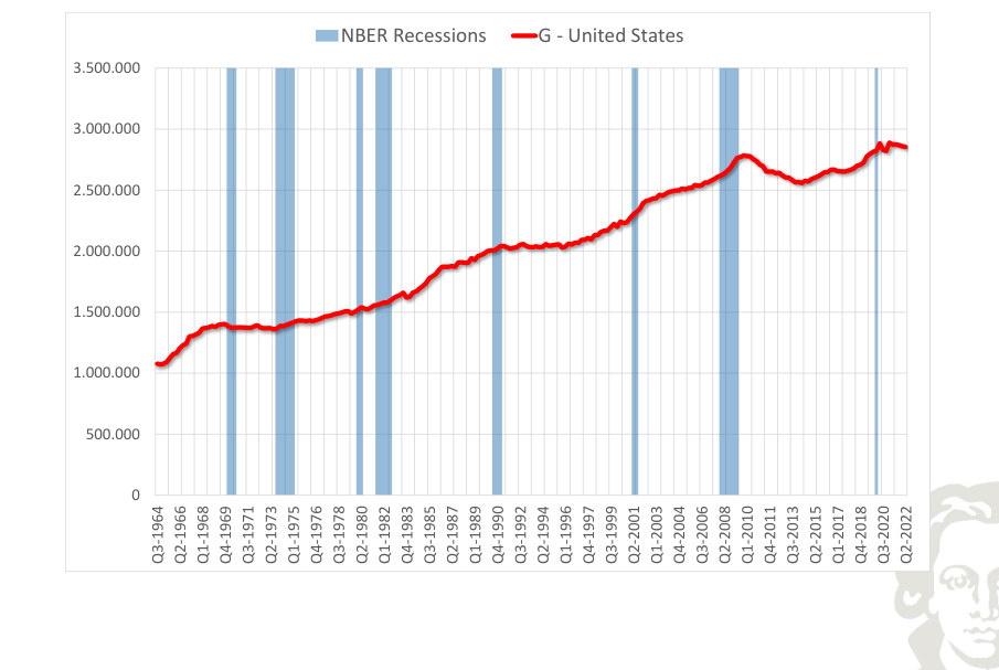
NBER Recessions G - United States (Annual Growth)

**Figure 42.** United States: government expenditure, growth rate, with recession shading.

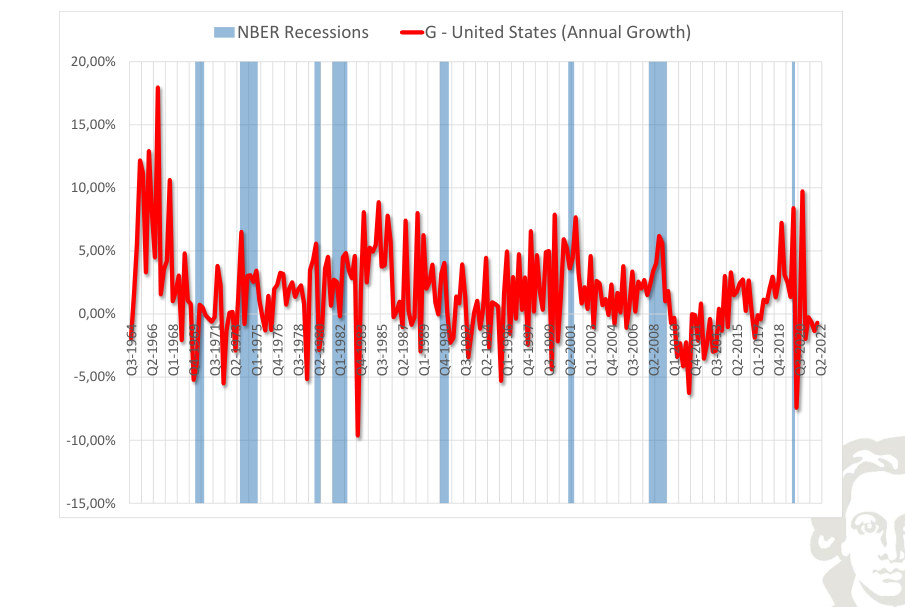
The plotted growth rate of government expenditure for the United States measures the change in activity under the frequency and rate convention of the series. Negative growth and below-trend growth are different concepts; comparing them helps identify contractions without assuming that every slowing constitutes a recession.

NBER Recessions G - United States (Annual Trend Growth)

**Figure 43.** United States: government expenditure, smoothed trend growth, with recession shading.

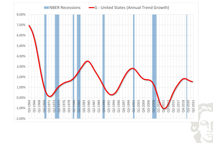
The smoothed growth path of government expenditure in the United States describes the slower-moving change in the rate of expansion. It should not be equated with the cyclical component: the trend-growth series may slow even when the level of activity continues to rise.

NBER Recessions G - United States (Deviations from Trend)

**Figure 44.** United States: government expenditure, deviation from trend, with recession shading.

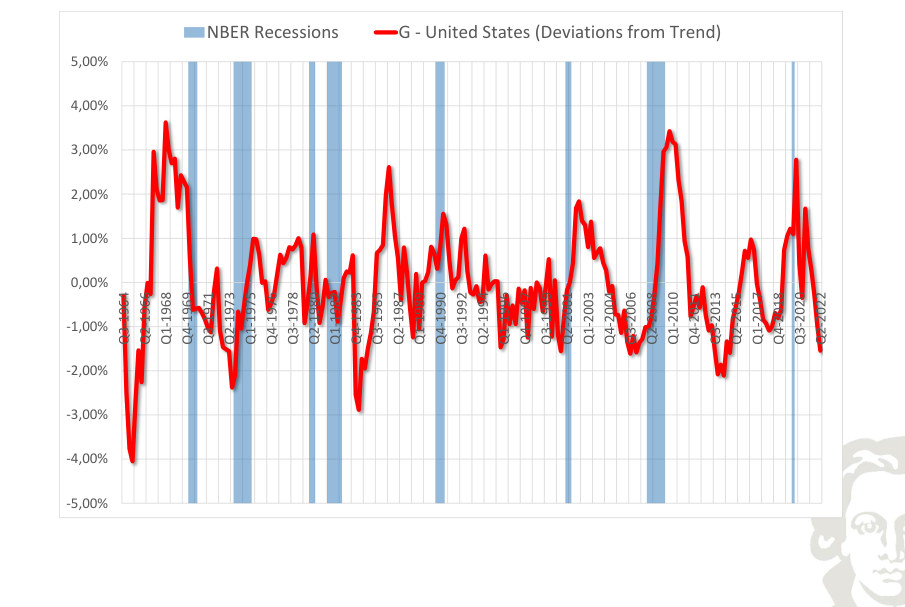
Detrended government expenditure for the United States highlights movements above and below the estimated long-run path. The horizontal zero line is a normalization relative to the chosen filter, not a literal condition of zero production. Compare the timing and amplitude of these fluctuations with the corresponding output series.

NBER Recessions X - United States

**Figure 45.** United States: exports, level, with recession shading.

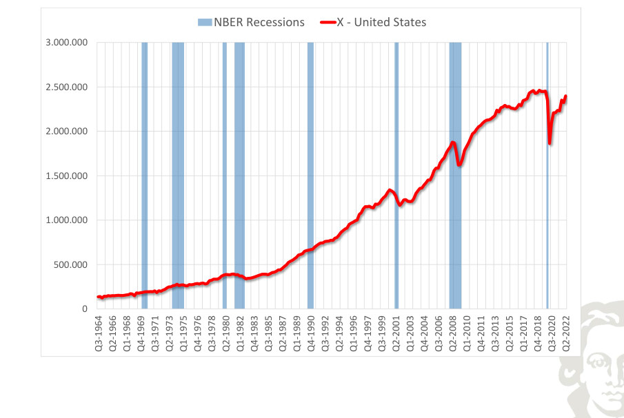
NBER Recessions X - United States (Annual Growth)

**Figure 46.** United States: exports, growth rate, with recession shading.

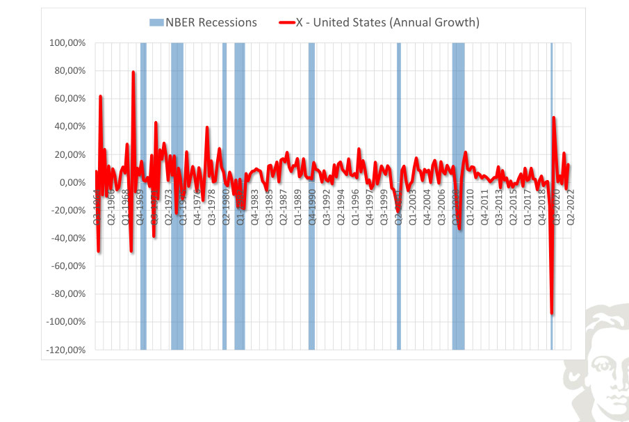
The plotted growth rate of exports for the United States measures the change in activity under the frequency and rate convention of the series. Negative growth and below-trend growth are different concepts; comparing them helps identify contractions without assuming that every slowing constitutes a recession.

NBER Recessions X - United States (Annual Trend Growth)

**Figure 47.** United States: exports, smoothed trend growth, with recession shading.

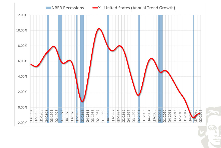
The smoothed growth path of exports in the United States describes the slower-moving change in the rate of expansion. It should not be equated with the cyclical component: the trend-growth series may slow even when the level of activity continues to rise.

NBER Recessions X - United States (Deviations from Trend)

**Figure 48.** United States: exports, deviation from trend, with recession shading.

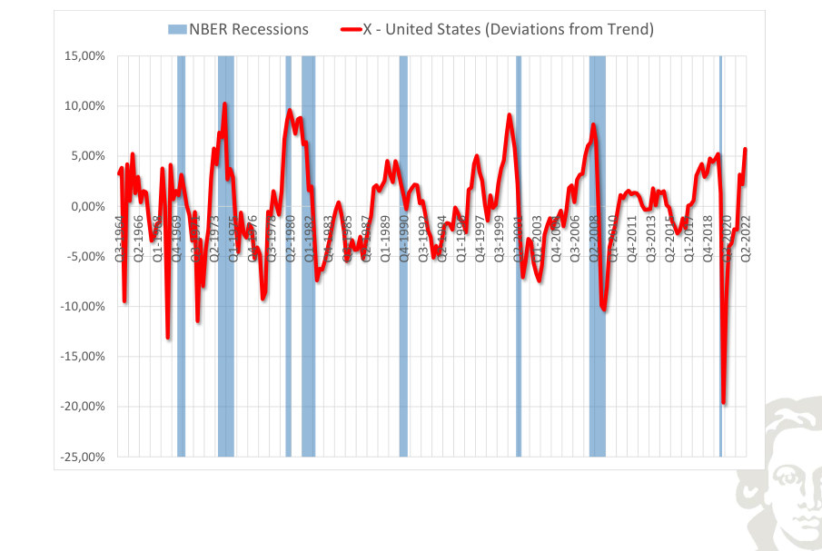
Detrended exports for the United States highlights movements above and below the estimated long-run path. The horizontal zero line is a normalization relative to the chosen filter, not a literal condition of zero production. Compare the timing and amplitude of these fluctuations with the corresponding output series.

NBER Recessions Z - United States

**Figure 49.** United States: imports, level, with recession shading.

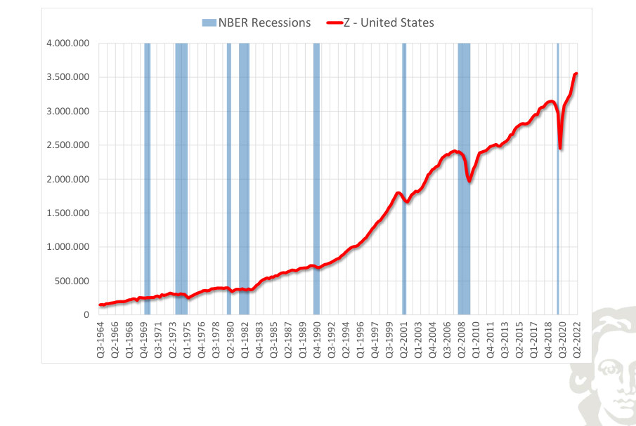
NBER Recessions Z - United States (Annual Growth)

**Figure 50.** United States: imports, growth rate, with recession shading.

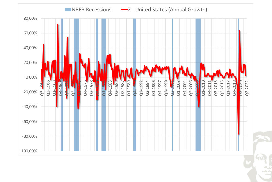
The plotted growth rate of imports for the United States measures the change in activity under the frequency and rate convention of the series. Negative growth and below-trend growth are different concepts; comparing them helps identify contractions without assuming that every slowing constitutes a recession.

NBER Recessions Z - United States (Annual Trend Growth)

**Figure 51.** United States: imports, smoothed trend growth, with recession shading.

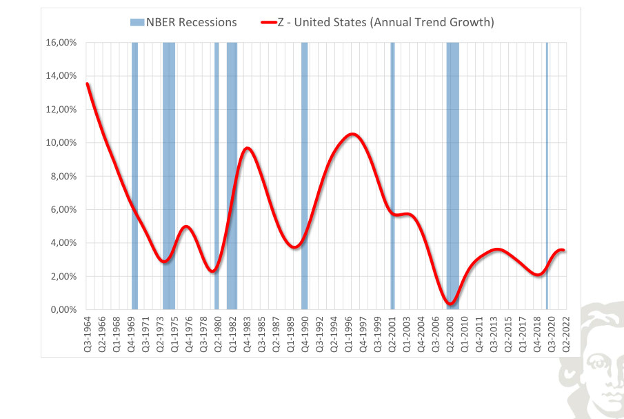
The smoothed growth path of imports in the United States describes the slower-moving change in the rate of expansion. It should not be equated with the cyclical component: the trend-growth series may slow even when the level of activity continues to rise.

NBER Recessions Z - United States (Deviations from Trend)

**Figure 52.** United States: imports, deviation from trend, with recession shading.

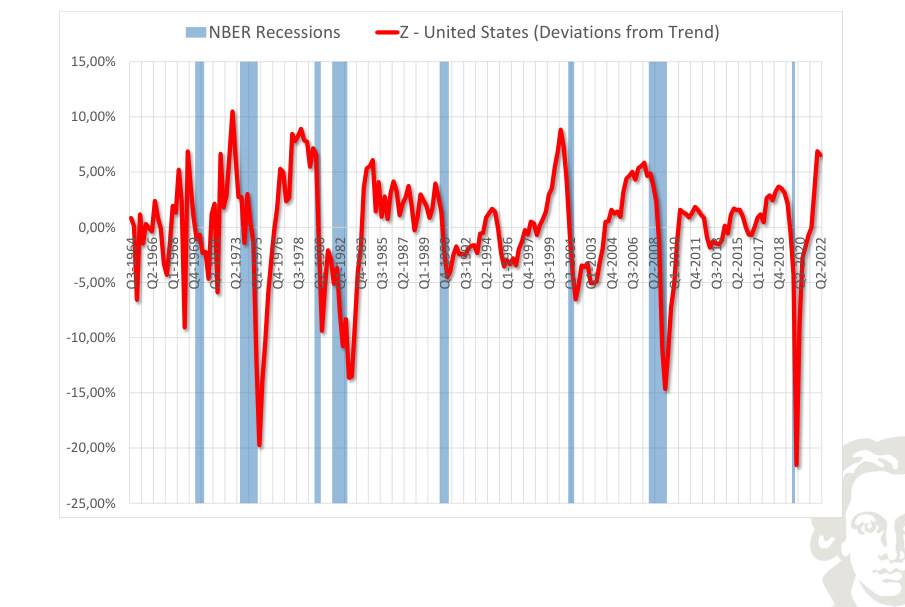
Detrended imports for the United States highlights movements above and below the estimated long-run path. The horizontal zero line is a normalization relative to the chosen filter, not a literal condition of zero production. Compare the timing and amplitude of these fluctuations with the corresponding output series.

EU (18) · country series

CEPR Y - Euro area

**Figure 53.** Euro area: output, level, with recession shading.

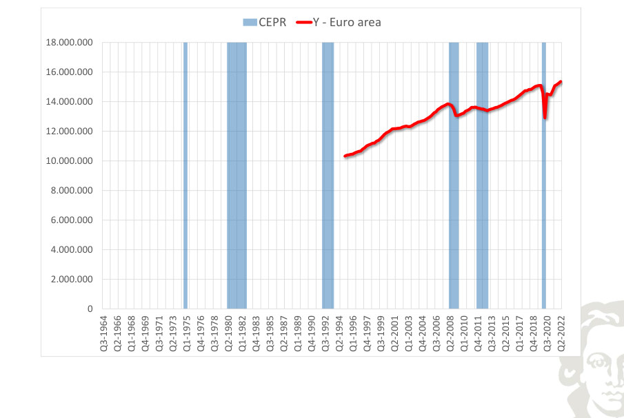
CEPR Y - Euro area (Annual Growth)

**Figure 54.** Euro area: output, growth rate, with recession shading.

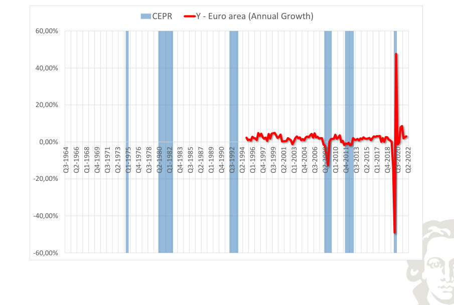
The plotted growth rate of real output for the selected economy measures the change in activity under the frequency and rate convention of the series. Negative growth and below-trend growth are different concepts; comparing them helps identify contractions without assuming that every slowing constitutes a recession.

CEPR Y - Euro area (Annual Trend Growth)

**Figure 55.** Euro area: output, smoothed trend growth, with recession shading.

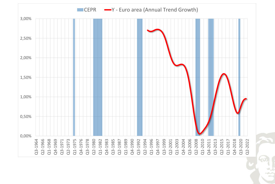
The smoothed growth path of real output in the selected economy describes the slower-moving change in the rate of expansion. It should not be equated with the cyclical component: the trend-growth series may slow even when the level of activity continues to rise.

CEPR Y - Euro area (Deviations from Trend)

**Figure 56.** Euro area: output, deviation from trend, with recession shading.

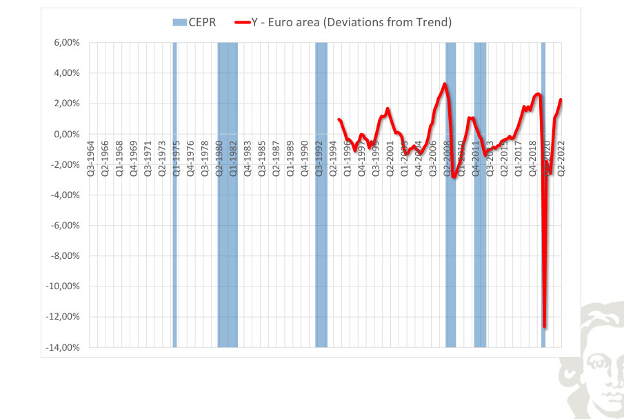
Detrended real output for the selected economy highlights movements above and below the estimated long-run path. The horizontal zero line is a normalization relative to the chosen filter, not a literal condition of zero production. Compare the timing and amplitude of these fluctuations with the corresponding output series.

CEPR C - Euro area

**Figure 57.** Euro area: consumption, level, with recession shading.

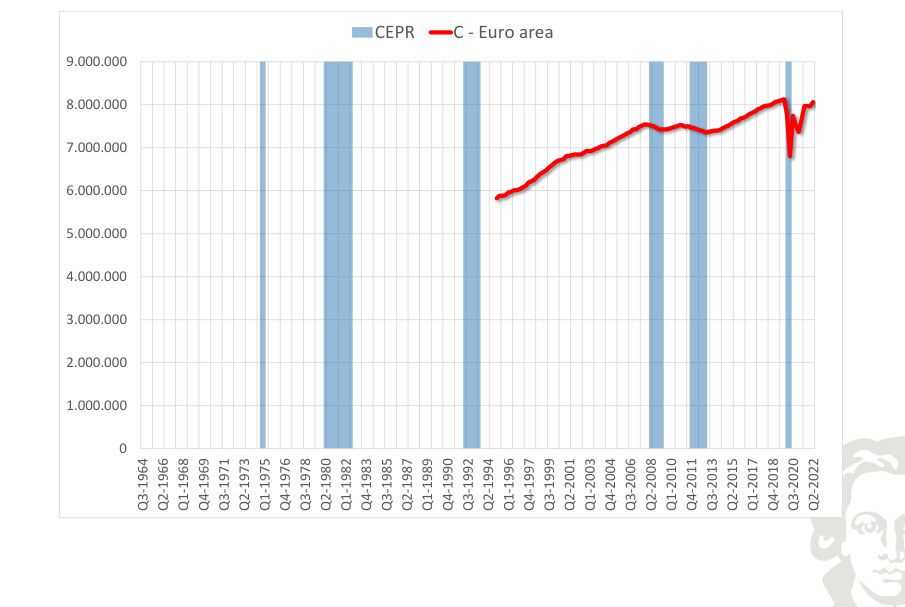
CEPR C - Euro area (Annual Growth)

**Figure 58.** Euro area: consumption, growth rate, with recession shading.

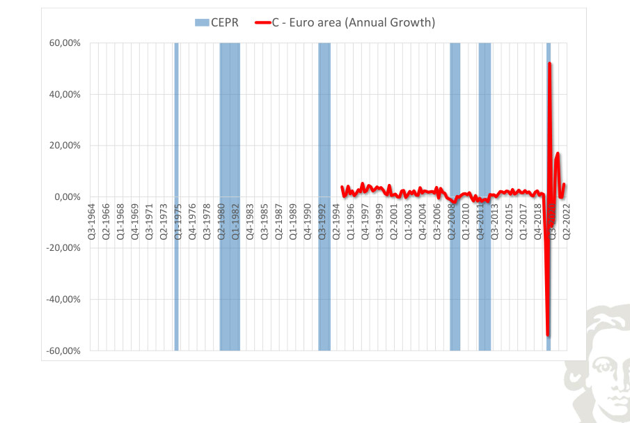
The plotted growth rate of consumption for the selected economy measures the change in activity under the frequency and rate convention of the series. Negative growth and below-trend growth are different concepts; comparing them helps identify contractions without assuming that every slowing constitutes a recession.

CEPR C - Euro area (Annual Trend Growth)

**Figure 59.** Euro area: consumption, smoothed trend growth, with recession shading.

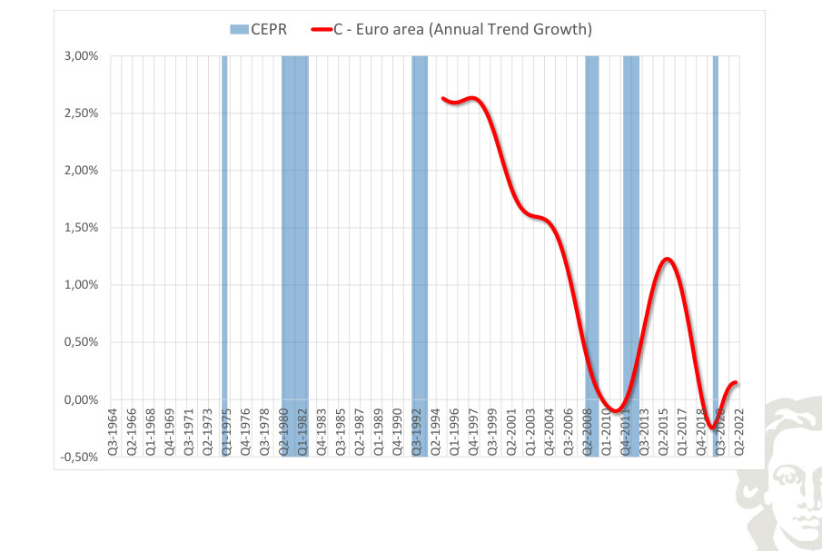
The smoothed growth path of consumption in the selected economy describes the slower-moving change in the rate of expansion. It should not be equated with the cyclical component: the trend-growth series may slow even when the level of activity continues to rise.

CEPR C - Euro Area (Deviations from Trend)

**Figure 60.** Euro area: consumption, deviation from trend, with recession shading.

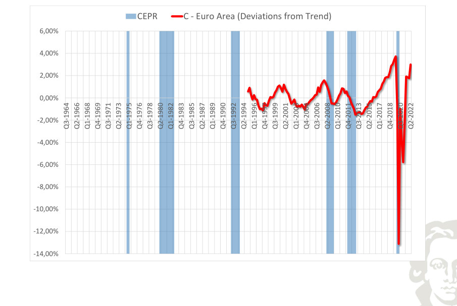
Detrended consumption for the selected economy highlights movements above and below the estimated long-run path. The horizontal zero line is a normalization relative to the chosen filter, not a literal condition of zero production. Compare the timing and amplitude of these fluctuations with the corresponding output series.

CEPR I - Euro area

**Figure 61.** Euro area: investment, level, with recession shading.

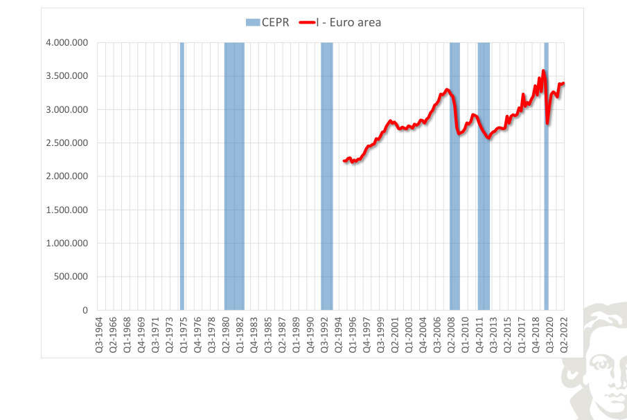
CEPR I - Euro area (Annual Growth)

**Figure 62.** Euro area: investment, growth rate, with recession shading.

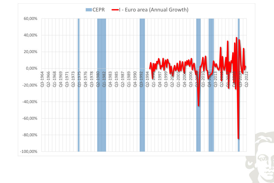
The plotted growth rate of investment for the selected economy measures the change in activity under the frequency and rate convention of the series. Negative growth and below-trend growth are different concepts; comparing them helps identify contractions without assuming that every slowing constitutes a recession.

CEPR I - Euro area (Annual Trend Growth)

**Figure 63.** Euro area: investment, smoothed trend growth, with recession shading.

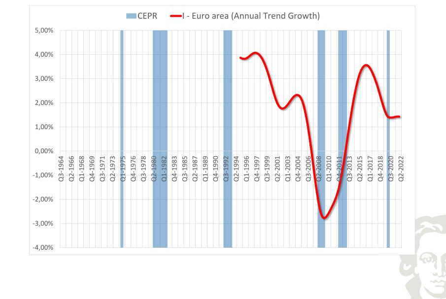
The smoothed growth path of investment in the selected economy describes the slower-moving change in the rate of expansion. It should not be equated with the cyclical component: the trend-growth series may slow even when the level of activity continues to rise.

CEPR I - Euro Area (Deviations from Trend)

**Figure 64.** Euro area: investment, deviation from trend, with recession shading.

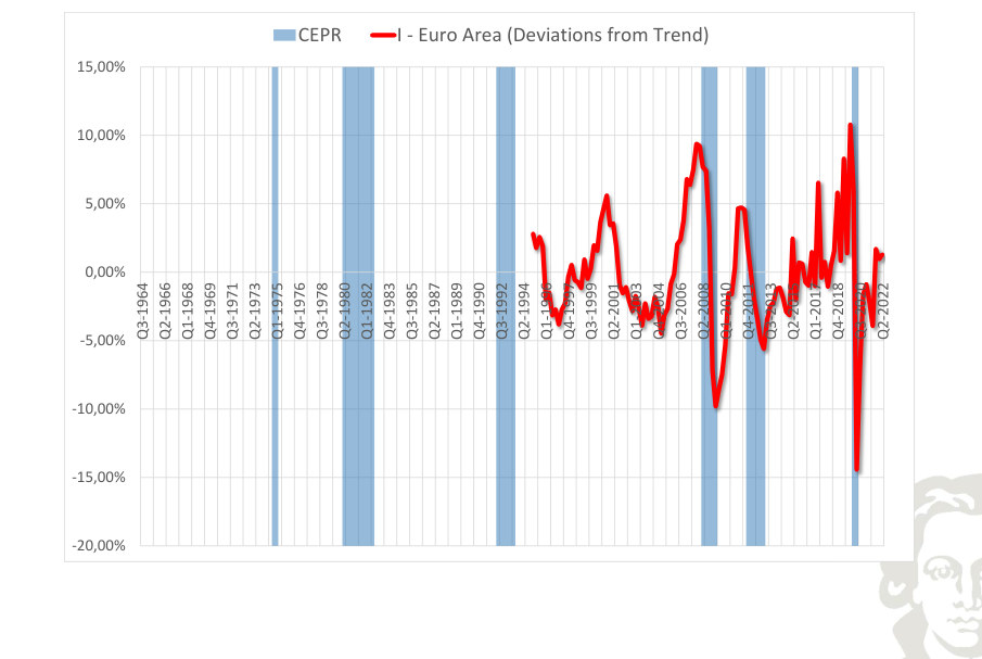
Detrended investment for the selected economy highlights movements above and below the estimated long-run path. The horizontal zero line is a normalization relative to the chosen filter, not a literal condition of zero production. Compare the timing and amplitude of these fluctuations with the corresponding output series.

CEPR G - Euro area

**Figure 65.** Euro area: government expenditure, level, with recession shading.

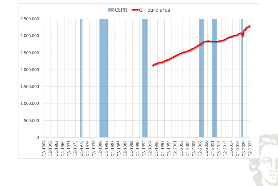
CEPR G - Euro area (Annual Growth)

**Figure 66.** Euro area: government expenditure, growth rate, with recession shading.

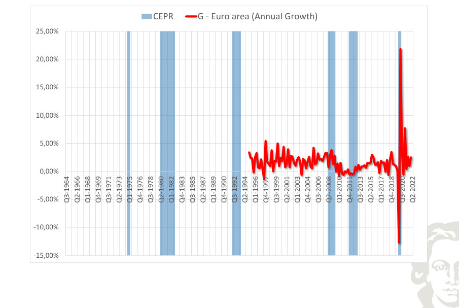
The plotted growth rate of government expenditure for the selected economy measures the change in activity under the frequency and rate convention of the series. Negative growth and below-trend growth are different concepts; comparing them helps identify contractions without assuming that every slowing constitutes a recession.

CEPR G - Euro area (Annual Trend Growth)

**Figure 67.** Euro area: government expenditure, smoothed trend growth, with recession shading.

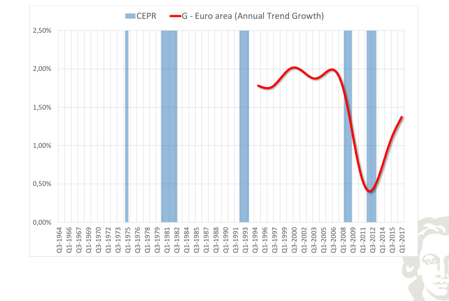
The smoothed growth path of government expenditure in the selected economy describes the slower-moving change in the rate of expansion. It should not be equated with the cyclical component: the trend-growth series may slow even when the level of activity continues to rise.

CEPR G - Euro area (Deviations from Trend)

**Figure 68.** Euro area: government expenditure, deviation from trend, with recession shading.

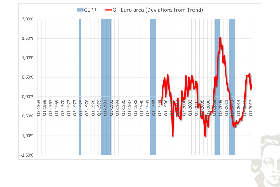
Detrended government expenditure for the selected economy highlights movements above and below the estimated long-run path. The horizontal zero line is a normalization relative to the chosen filter, not a literal condition of zero production. Compare the timing and amplitude of these fluctuations with the corresponding output series.

Japan · country series

OECD Japan Y - Japan

**Figure 69.** Japan: output, level, with recession shading.

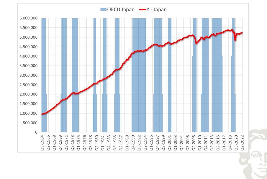
OECD Japan Y - Japan (Annual Growth)

**Figure 70.** Japan: output, growth rate, with recession shading.

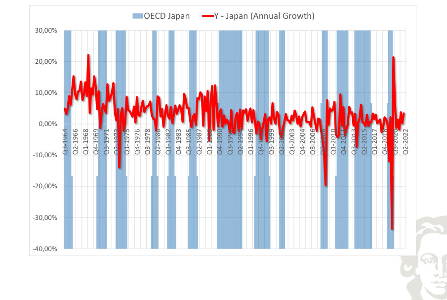
The plotted growth rate of real output for Japan measures the change in activity under the frequency and rate convention of the series. Negative growth and below-trend growth are different concepts; comparing them helps identify contractions without assuming that every slowing constitutes a recession.

OECD Japan Y - Japan (Annual Trend Growth)

**Figure 71.** Japan: output, smoothed trend growth, with recession shading.

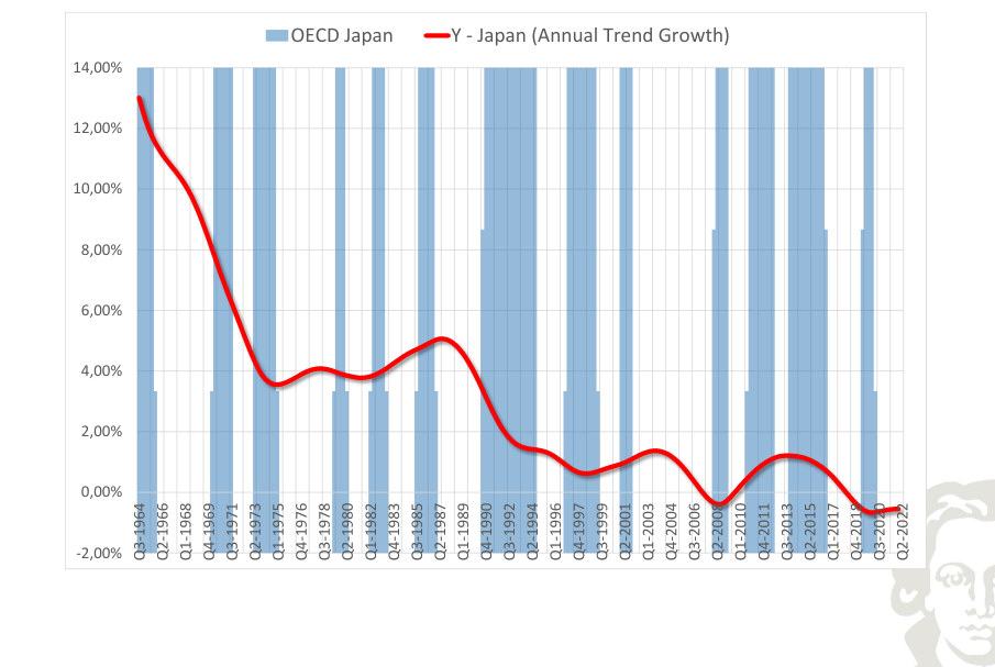
The smoothed growth path of real output in Japan describes the slower-moving change in the rate of expansion. It should not be equated with the cyclical component: the trend-growth series may slow even when the level of activity continues to rise.

OECD Japan Y - Japan (Deviations from Trend)

**Figure 72.** Japan: output, deviation from trend, with recession shading.

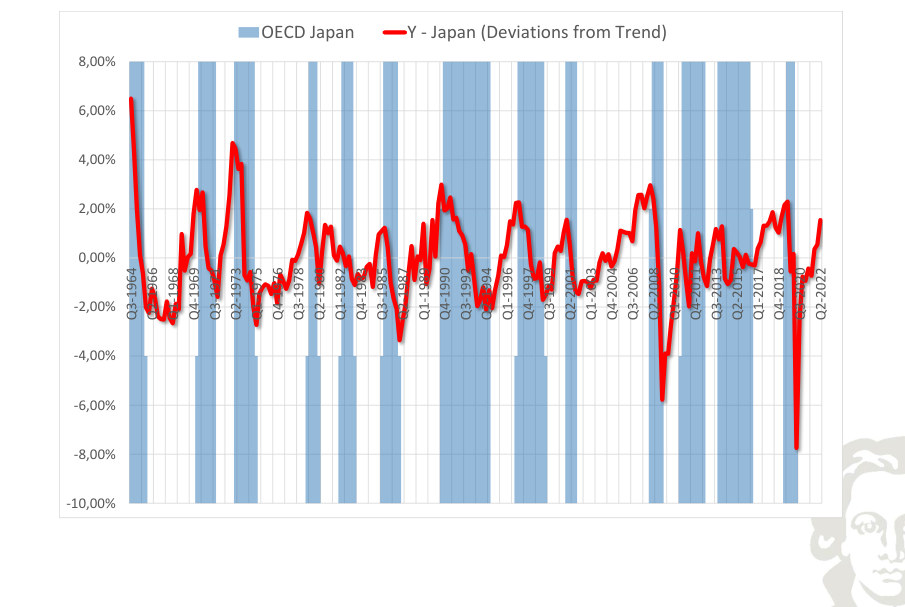
Detrended real output for Japan highlights movements above and below the estimated long-run path. The horizontal zero line is a normalization relative to the chosen filter, not a literal condition of zero production. Compare the timing and amplitude of these fluctuations with the corresponding output series.

OECD Japan C - Japan

**Figure 73.** Japan: consumption, level, with recession shading.

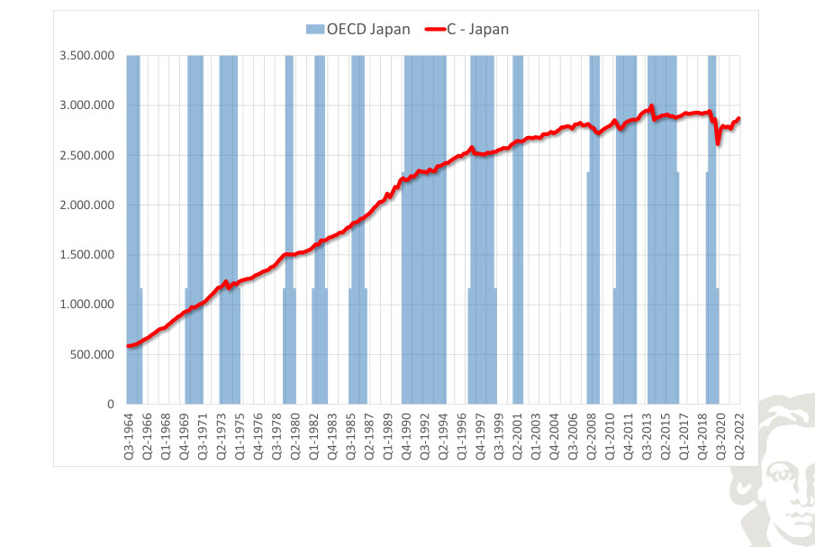
OECD Japan C - Japan (Annual Growth)

**Figure 74.** Japan: consumption, growth rate, with recession shading.

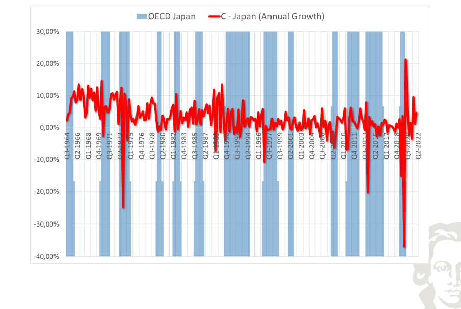
The plotted growth rate of consumption for Japan measures the change in activity under the frequency and rate convention of the series. Negative growth and below-trend growth are different concepts; comparing them helps identify contractions without assuming that every slowing constitutes a recession.

OECD Japan C - Japan (Annual Trend Growth)

**Figure 75.** Japan: consumption, smoothed trend growth, with recession shading.

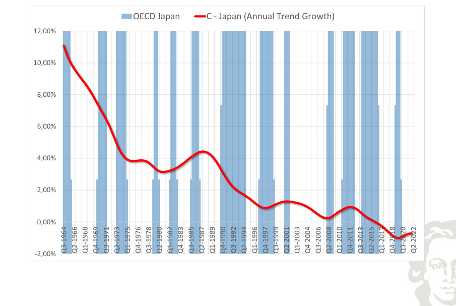
The smoothed growth path of consumption in Japan describes the slower-moving change in the rate of expansion. It should not be equated with the cyclical component: the trend-growth series may slow even when the level of activity continues to rise.

OECD Japan C - Japan (Deviations from Trend)

**Figure 76.** Japan: consumption, deviation from trend, with recession shading.

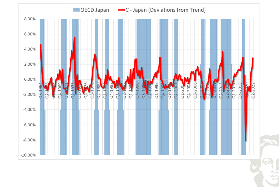
Detrended consumption for Japan highlights movements above and below the estimated long-run path. The horizontal zero line is a normalization relative to the chosen filter, not a literal condition of zero production. Compare the timing and amplitude of these fluctuations with the corresponding output series.

OECD Japan I - Japan

**Figure 77.** Japan: investment, level, with recession shading.

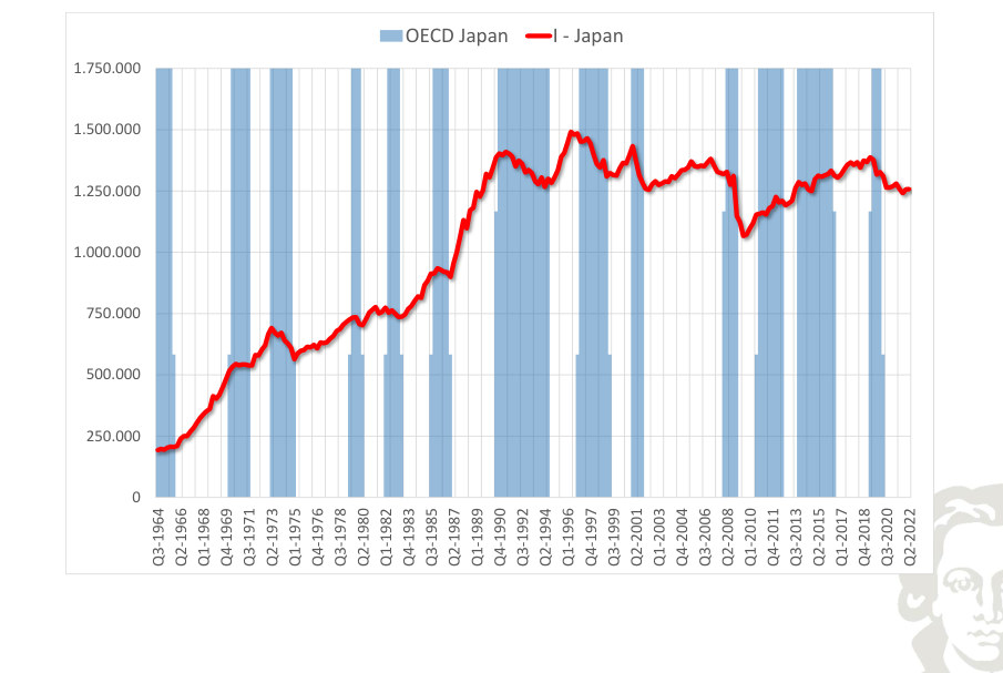
OECD Japan I - Japan (Annual Growth)

**Figure 78.** Japan: investment, growth rate, with recession shading.

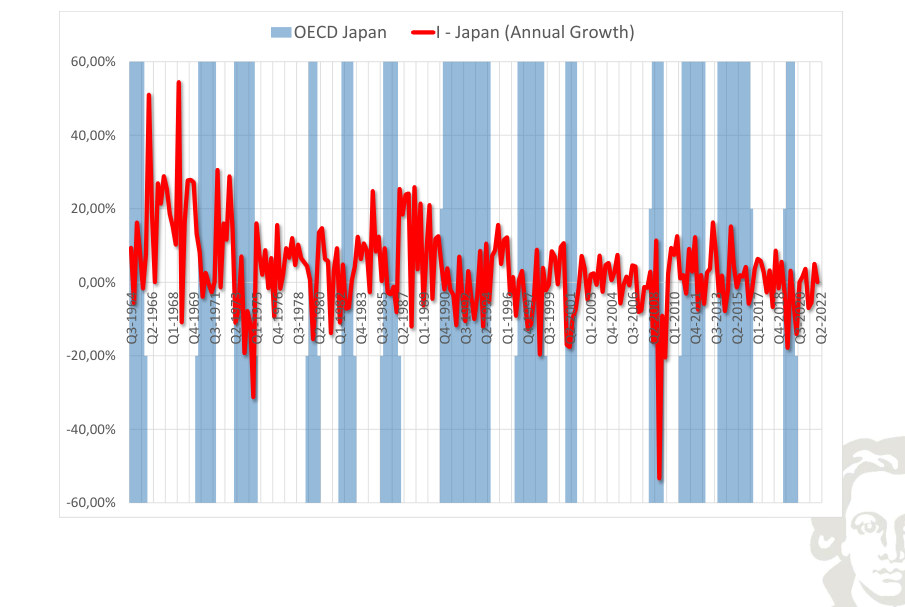
The plotted growth rate of investment for Japan measures the change in activity under the frequency and rate convention of the series. Negative growth and below-trend growth are different concepts; comparing them helps identify contractions without assuming that every slowing constitutes a recession.

OECD Japan I - Japan (Annual Trend Growth)

**Figure 79.** Japan: investment, smoothed trend growth, with recession shading.

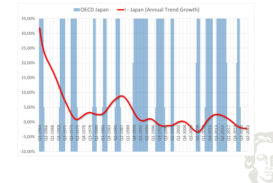
The smoothed growth path of investment in Japan describes the slower-moving change in the rate of expansion. It should not be equated with the cyclical component: the trend-growth series may slow even when the level of activity continues to rise.

OECD Japan I - Japan (Deviations from Trend)

**Figure 80.** Japan: investment, deviation from trend, with recession shading.

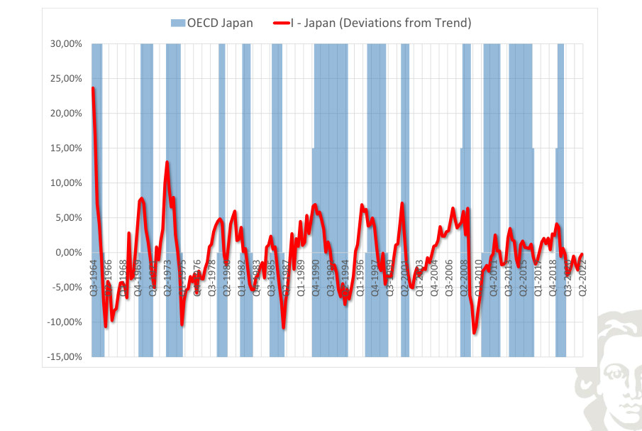
Detrended investment for Japan highlights movements above and below the estimated long-run path. The horizontal zero line is a normalization relative to the chosen filter, not a literal condition of zero production. Compare the timing and amplitude of these fluctuations with the corresponding output series.

OECD Japan G - Japan

**Figure 81.** Japan: government expenditure, level, with recession shading.

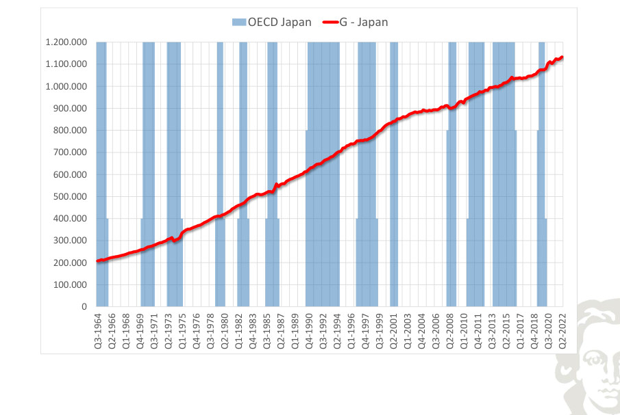
OECD Japan G - Japan (Annual Growth)

**Figure 82.** Japan: government expenditure, growth rate, with recession shading.

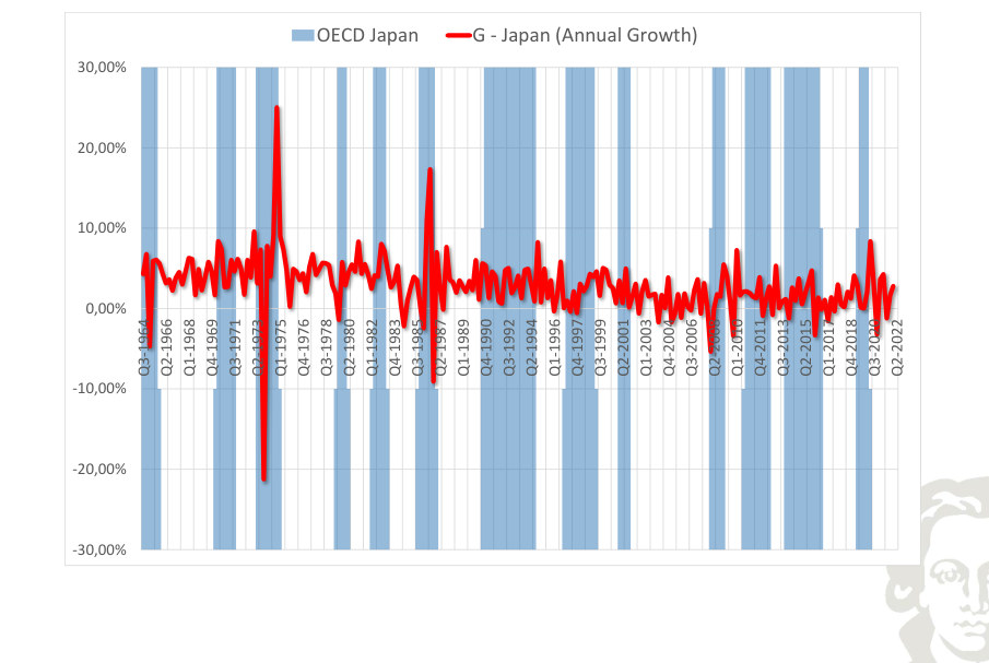
The plotted growth rate of government expenditure for Japan measures the change in activity under the frequency and rate convention of the series. Negative growth and below-trend growth are different concepts; comparing them helps identify contractions without assuming that every slowing constitutes a recession.

OECD Japan G - Japan (Annual Trend Growth)

**Figure 83.** Japan: government expenditure, smoothed trend growth, with recession shading.

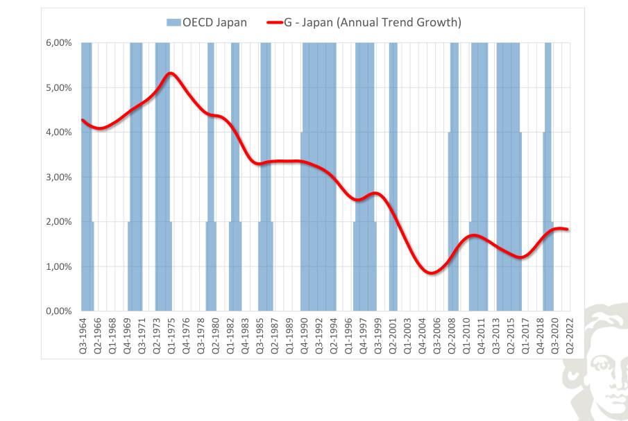
The smoothed growth path of government expenditure in Japan describes the slower-moving change in the rate of expansion. It should not be equated with the cyclical component: the trend-growth series may slow even when the level of activity continues to rise.

OECD Japan G - Japan (Deviations from Trend)

**Figure 84.** Japan: government expenditure, deviation from trend, with recession shading.

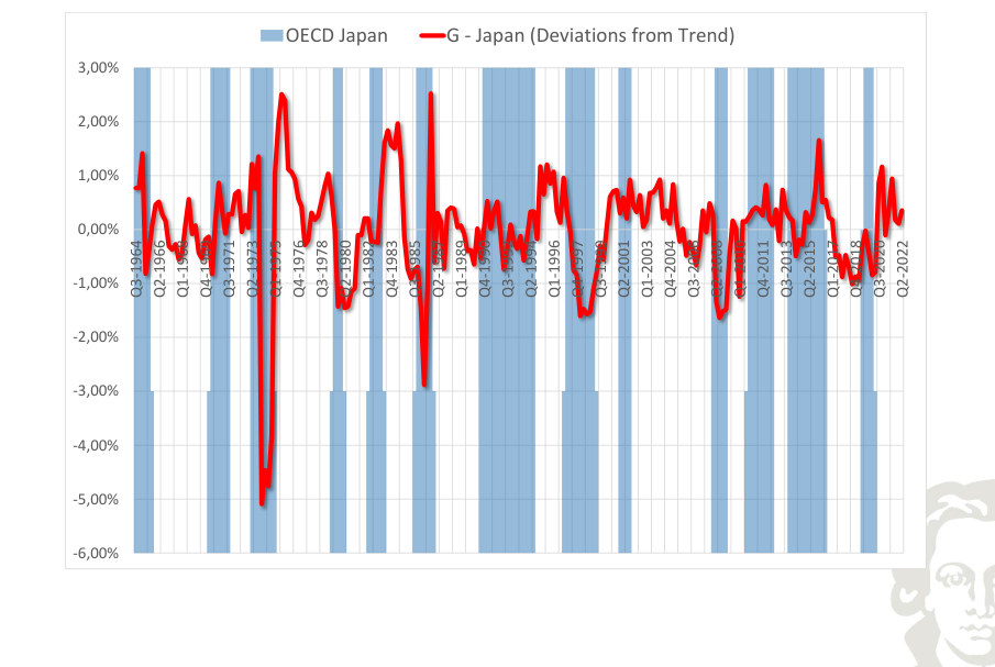
Detrended government expenditure for Japan highlights movements above and below the estimated long-run path. The horizontal zero line is a normalization relative to the chosen filter, not a literal condition of zero production. Compare the timing and amplitude of these fluctuations with the corresponding output series.

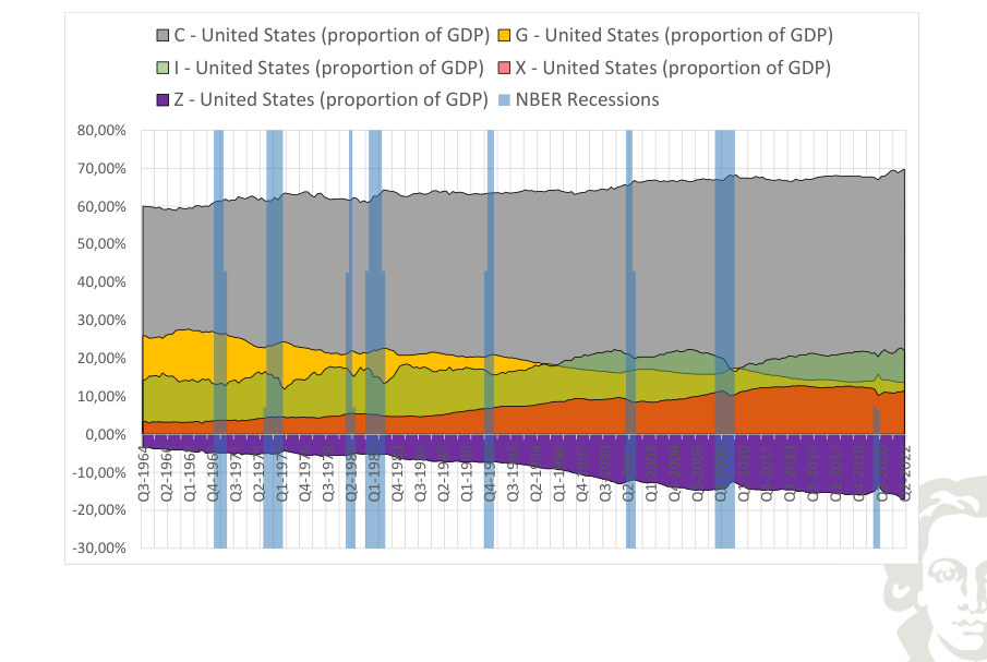
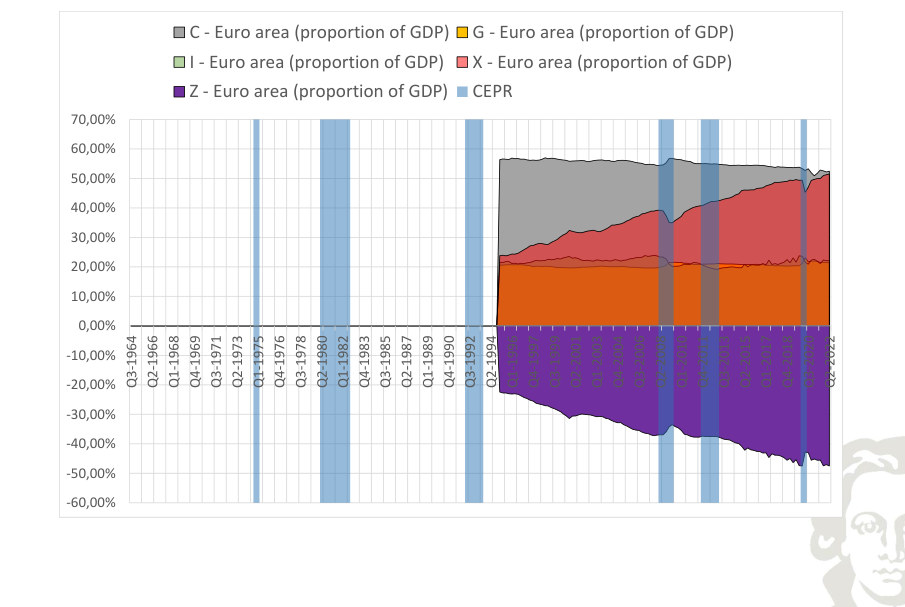
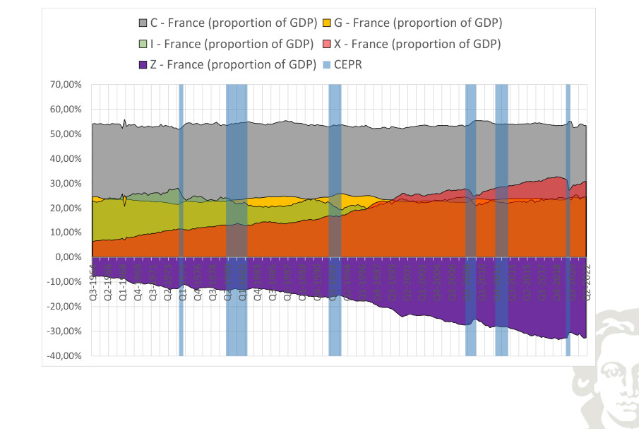
GDP Ratios

Expenditure components can be expressed relative to GDP to compare their importance across time and economies:

\frac{C_{t}}{Y_{t}}, \frac{G_{t}}{Y_{t}}, \frac{I_{t}}{Y_{t}}, \frac{X_{t}}{Y_{t}}, \frac{I M_{t}}{Y_{t}}

Some aggregate expenditure ratios are relatively stable over long horizons. The country plots use OECD data.

C - United States (proportion of GDP) G - United States (proportion of GDP)

**Figure 85.** United States: expenditure components as shares of GDP; imports enter with a negative sign.

C - Euro area (proportion of GDP) G - Euro area (proportion of GDP)

**Figure 86.** Euro area: expenditure components as shares of GDP; imports enter with a negative sign.

C - France (proportion of GDP) G - France (proportion of GDP)

**Figure 87.** France: expenditure components as shares of GDP; imports enter with a negative sign.

C - Germany (proportion of GDP) I - Germany (proportion of GDP)

**Figure 88.** Germany: expenditure components as shares of GDP; imports enter with a negative sign.

C - Italy (proportion of GDP) G- Italy (proportion of GDP)

**Figure 89.** Italy: expenditure components as shares of GDP; imports enter with a negative sign.

C - Japan (proportion of GDP) G - Japan (proportion of GDP)

**Figure 90.** Japan: expenditure components as shares of GDP; imports enter with a negative sign.

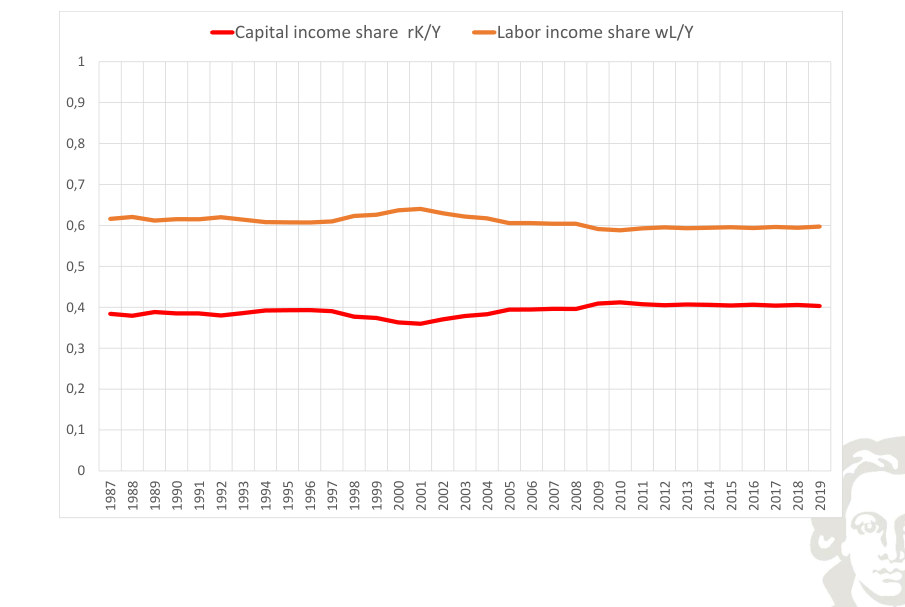
Kaldor Stylized Facts

Balanced growth concerns stable long-run ratios and trends, whereas cyclical statistics describe deviations around those trends. Both are useful targets for a quantitative economic model, but they should not be conflated.

A volatility statistic summarizes the typical amplitude of fluctuations; a correlation describes direction and timing of comovement. Dividing a variable's standard deviation by output's standard deviation produces a scale-free relative volatility. Comparing those moments for simulated and observed data provides a model-diagnostic rather than a proof of causality.

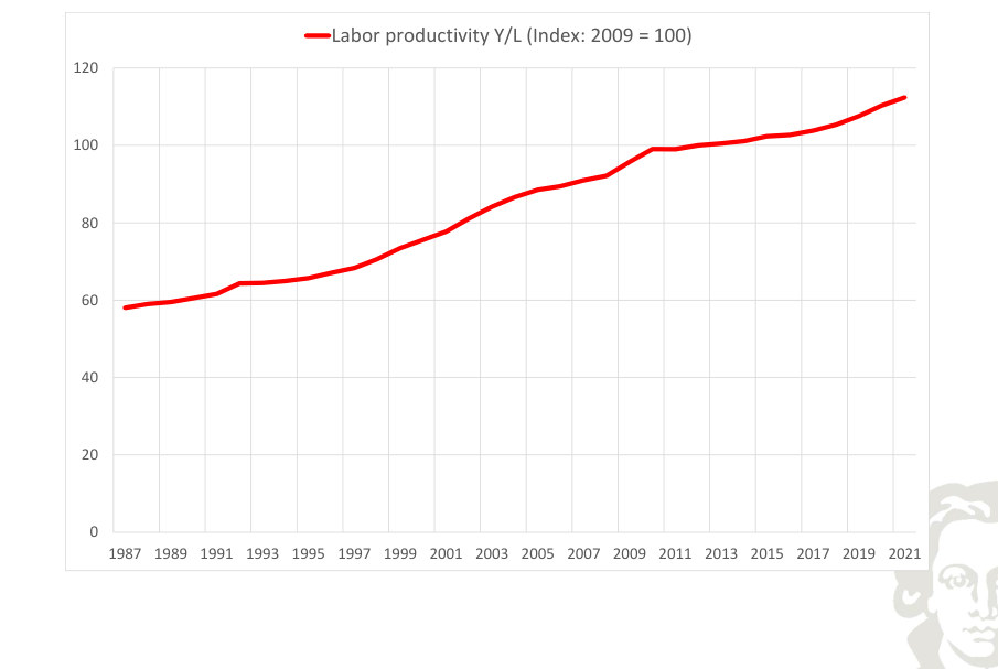
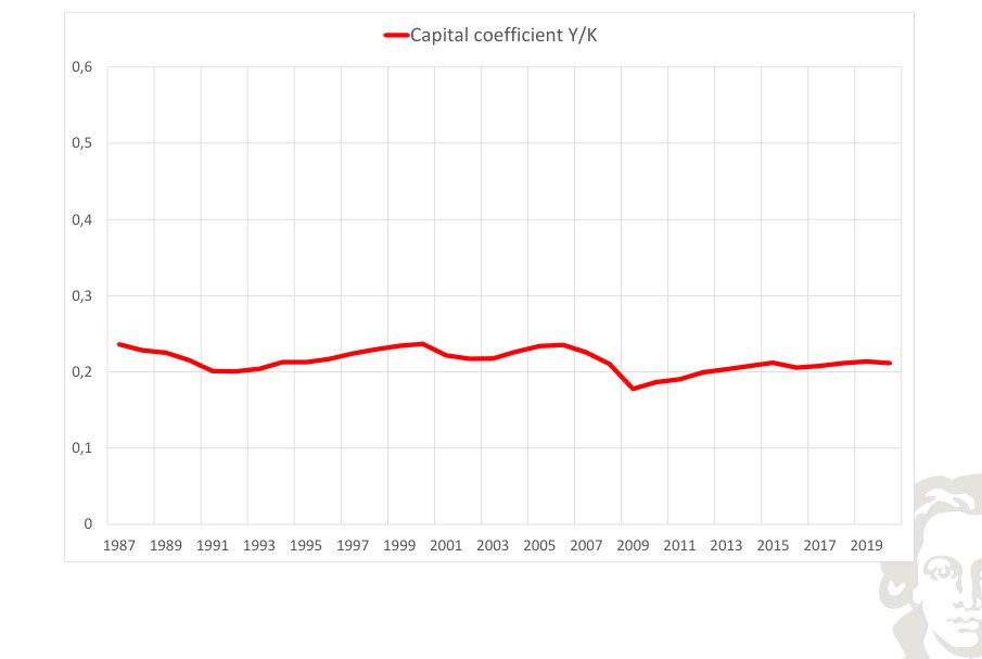
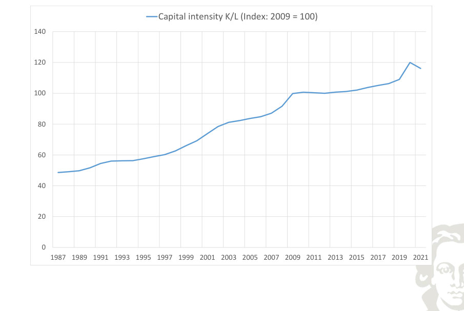
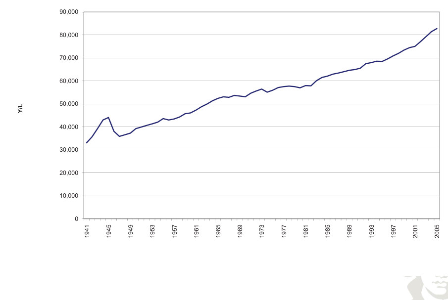
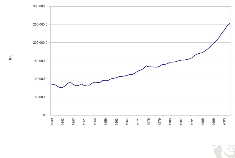
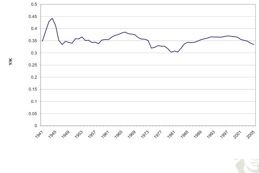
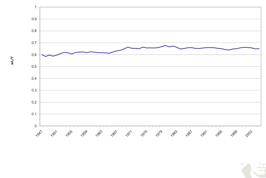
Kaldor’s balanced-growth regularities concern rising output per worker Y/L and capital per worker K/L, a comparatively stable return on capital, a comparatively stable capital–output ratio K/Y, and comparatively stable labor and capital income shares wL/Y and rK/Y. These are long-run regularities rather than exact laws for every sample.

Capital income share rK/Y Labor income share wL/Y

**Figure 91.** Capital and labor income shares over time.

Labor productivity Y/L (Index: 2009 = 100)

**Figure 92.** Labor productivity, output per unit of labor.

Capital coefficient Y/K

**Figure 93.** Output-to-capital ratio over time.

Capital intensity K/L (Index: 2009 = 100)

**Figure 94.** Capital intensity, capital per unit of labor.

90,000

**Figure 95.** Historical series for output per unit of labor.

300,000.0

**Figure 96.** Historical series for capital per unit of labor.

5

**Figure 97.** Historical output-to-capital ratio.

1

**Figure 98.** Historical labor-income share.

Solow Model

Capital accumulation creates an intertemporal trade-off: resources devoted to investment raise future productive capacity but reduce resources left for present consumption. In the Solow model the saving fraction is imposed; a steady-state capital stock balances depreciation and effective-labor growth against investment. The Golden Rule savings rate maximizes steady-state consumption, but a structural policy analysis should allow individuals to adjust their saving behavior.

The Solow model expresses output per effective worker as y = k^θ. On its balanced growth path, k and y are constant, while output and capital per worker grow at the rate of labor-augmenting technical progress.

Quantity	Balanced-growth behavior
K/(AL)	Constant
Y/(AL)	Constant
K/L and Y/L	Grow with A
L	Grows with population
K and Y	Grow with effective labor AL
Y/K	Constant

In discrete time the gross growth factor of aggregate capital and output is (1+g_A)(1+g_L). The sum g_A+g_L is a first-order approximation. Source: Blanchard and Illing, Macroeconomics, balanced-growth discussion.

Companies

Competitive firms hire capital and labor until their marginal products equal factor prices. With labor-augmenting Cobb–Douglas technology:

Y_{t} = {(A_{t} L_{t})}^{1 - θ} K_{t - 1}^{θ}

w_{t} = (1 - θ) \frac{Y_{t}}{L_{t}}, r_{t} = θ \frac{Y_{t}}{K_{t - 1}}

A constant capital-to-effective-labor ratio implies a constant capital rental return along the balanced growth path.

Kaldor Facts 5

Competitive Cobb–Douglas factor prices imply labor income wₜLₜ/Yₜ = 1−θ and capital income rₜKₜ₋₁/Yₜ = θ. These constant shares follow from the Cobb–Douglas elasticities together with marginal-product pricing. Constant returns and competition alone imply that factor payments exhaust output; they do not imply constant individual shares for every production function.

Critical Appraisal Of Solow

The Solow model explains growth and capital transition dynamics with an imposed saving rate. It cannot determine how optimal saving changes when taxes, returns or expectations change, because it lacks a household intertemporal optimization problem. This limitation concerns endogenous forward-looking behavior, not the absence of dynamics: the capital accumulation equation is itself dynamic.

Forward-looking households may increase current consumption when they anticipate higher future resources. A model with intertemporal optimization can explain how such expectations influence present saving and consumption.

Decomposing observed macroeconomic data

Data Transformations

Average hours equal total hours divided by employment; labor productivity equals real output divided by hours. A capital series can be built from investment and a stated initial stock using the perpetual-inventory equation:

k_{t} = (1 - δ) k_{t - 1} + i_{t}

The initial stock can be independently measured or approximated by i₀/δ under a no-growth steady-state assumption. With Cobb–Douglas production, the log productivity residual is:

log A_{t} = log Y_{t} - θ log k_{t - 1} - (1 - θ) log ℓ_{t}

The illustrative data construction uses δ = 0.03 and a labor-income share near 0.67. These choices differ from the later benchmark calibration and must remain tied to their respective empirical exercise.

Variability And Correlation

The empirical volatility table above reports log per-capita HP-filtered deviations. Consumption is less volatile than output, while investment is substantially more volatile. Ratios are based on unrounded source moments; dividing the displayed rounded standard deviations may not reproduce every ratio exactly.

Correlation

Empirical cross-correlations of log per-capita HP deviations, corr(Yₜ, xₜ₊ⱼ):

Series	-3	-2	-1	0	1	2	3
Output	0.369	0.581	0.776	1.000	0.776	0.581	0.369
Non-durable consumption	0.109	0.298	0.564	0.701	0.494	0.356	0.195
Investment	0.365	0.553	0.719	0.889	0.733	0.538	0.339
Capital	-0.260	-0.155	-0.018	0.155	0.370	0.535	0.645
Total hours	-0.086	0.055	0.229	0.429	0.626	0.881	0.786
Employment	-0.143	-0.039	0.107	0.288	0.478	0.801	0.721
Average hours	0.333	0.512	0.678	0.772	0.684	0.581	0.414
Labor productivity	0.136	0.049	-0.065	-0.244	-0.418	-0.475	-0.500
TFP	0.471	0.627	0.753	0.875	0.550	0.301	0.055

Contemporaneous consumption, investment and TFP are strongly positively correlated with output in this sample. Lead–lag patterns differ across variables.

Synthesis

A model should reproduce clearly defined growth and cyclical facts using appropriately transformed, comparable economic series.

3. Measuring business cycles: empirical regularities

Introduction

Integrated theoretical explanation

Formal framework and essential relationships

Three concepts of cyclical data

Kaldor facts and cyclical moments must not be confused

Empirical business-cycle moments

Explanations, derivations and empirical applications

What Are Business Cycles?

Why The Cycle?

Decomposing observed macroeconomic data

NBER Recession Output (Nonfarm Business, Current Dollars, Index: 2012 = 100)

Linear Trend (In Logs)

NBER Recession

NBER Recession Output (Nonfarm Business, Constant Prices, Index: 2012 = 100)

NBER Recession

NBER Recession Deviations from trend

NBER Recession

A Statistical Method: Hodrick-Prescott Filter

NBER Recession

NBER Recession Output Per Person Nonfarm

HP Vs. Band Pass Filter

Stylized Macro Facts

USA · country series

NBER Recessions Y - United States

NBER Recessions Y - United States (Annual Growth)

NBER Recessions Y - United States (Annual Trend Growth)

NBER Recessions Y - United States (Deviations from Trend)

NBER Recessions C - United States

NBER Recessions C - United States (Annual Growth)

NBER Recessions C - United States (Annual Trend Growth)

NBER Recessions C - United States (Deviations from Trend)

NBER Recessions I - United States

NBER Recessions I - United States (Annual Growth)

NBER Recessions I - United States (Annual Trend Growth)

NBER Recessions I - United States (Deviations from Trend)

NBER Recessions G - United States

NBER Recessions G - United States (Annual Growth)

NBER Recessions G - United States (Annual Trend Growth)

NBER Recessions G - United States (Deviations from Trend)

NBER Recessions X - United States

NBER Recessions X - United States (Annual Growth)

NBER Recessions X - United States (Annual Trend Growth)

NBER Recessions X - United States (Deviations from Trend)

NBER Recessions Z - United States

NBER Recessions Z - United States (Annual Growth)

NBER Recessions Z - United States (Annual Trend Growth)

NBER Recessions Z - United States (Deviations from Trend)

EU (18) · country series

CEPR Y - Euro area

CEPR Y - Euro area (Annual Growth)

CEPR Y - Euro area (Annual Trend Growth)

CEPR Y - Euro area (Deviations from Trend)

CEPR C - Euro area

CEPR C - Euro area (Annual Growth)

CEPR C - Euro area (Annual Trend Growth)

CEPR C - Euro Area (Deviations from Trend)

CEPR I - Euro area

CEPR I - Euro area (Annual Growth)

CEPR I - Euro area (Annual Trend Growth)

CEPR I - Euro Area (Deviations from Trend)

CEPR G - Euro area

CEPR G - Euro area (Annual Growth)

CEPR G - Euro area (Annual Trend Growth)

CEPR G - Euro area (Deviations from Trend)

Japan · country series

OECD Japan Y - Japan

OECD Japan Y - Japan (Annual Growth)

OECD Japan Y - Japan (Annual Trend Growth)

OECD Japan Y - Japan (Deviations from Trend)

OECD Japan C - Japan

OECD Japan C - Japan (Annual Growth)

OECD Japan C - Japan (Annual Trend Growth)

OECD Japan C - Japan (Deviations from Trend)

OECD Japan I - Japan

OECD Japan I - Japan (Annual Growth)

OECD Japan I - Japan (Annual Trend Growth)

OECD Japan I - Japan (Deviations from Trend)

OECD Japan G - Japan

Un dubbio da chiarire?
Studiamolo insieme.